Fig. 1
Representative CT images of patient samples with both diffuse consolidation and mass-like fibrosis before and after stereotactic body radiotherapy [113]. Reprinted with permission from Int J Radiat Oncol Biol Phys, Vol. 84, Dunlap et al., Computed tomography-based anatomic assessment overestimates local tumor recurrence in patients with mass-like consolidation after stereotactic body radiotherapy for early-stage non-small cell lung cancer, p. 1074, Copyright (2012), with permission from Elsevier
Imaging as a Tool for Patient Screening
The importance of cancer screening has been highlighted in the recently published National Lung Cancer Screening Trial (NLST) by demonstrating a 20 % reduction in mortality with the use of low-dose helical CT as opposed to chest X-ray [114]. Screening has the potential to allow for early detection of lung cancer resulting in a phenomenon termed “stage migration.” Patients will potentially be diagnosed at an earlier stage and thus more likely cured with treatment. Unfortunately, current diagnostic tools have limitations. In a study by Ko et al. [115], a small nodule size of ≤5 mm in diameter (nodule detection sensitivity: ≤5 vs. >5 mm, 74 % vs. 82 %), ground-glass opacity nodules (nodule detection sensitivity: ground-glass opacity vs. solid, 65 % vs. 83 %), and lesion location (nodule detection sensitivity: central vs. peripheral, 61 % vs. 80 %) were shown to be major factors that contribute to the difficulty in detecting nodules. Nodule detection can be improved by advances in computer-aided detection (CAD) systems that are being developed and evaluated to provide a second perspective for nodule detection on CT. The use of CAD can help improve radiologist performance for the detection of unidentified lung cancers during lung cancer screening with CT [116, 117].
When interpreting findings from CT, radiologists must take multiple factors into account when determining whether or not a lesion is malignant or benign. Specific features that must be considered include nodule morphology, growth rate assessment, clinical features incorporated into a Bayesian analysis, hemodynamic characteristics on CT, and metabolic characteristics on 18F-FDG PET. Morphologic criteria allow for predicting the odds ratio of malignancy based on specific radiographic criteria: lobulated margin, a spiculated margin, and the absence of a satellite nodule [118]. Determination of growth rate over a 2-year period has also been shown to be a cost-effective and reliable method. Unfortunately, this method relies heavily on volumetric analysis of a nodule where current segmentation methods are unreliable [119]. Bayesian analysis combines individual probabilities of malignancy in order to estimate the overall odds favoring malignancy. These features include cavities of 16 mm in thickness, irregular or spiculated margin on CT scans, patient complaints of hemoptysis, a patient history of malignancy, patient age >70 years, nodule size of 21–30 mm in diameter, nodule growth rate of 7–465 days, an ill-defined nodule on chest radiographs, patient a current smoker, and nodules with indeterminate calcification on CT scans [120]. Evaluation of tumor vascular with dynamic helical CT has also been proven to be beneficial. Threshold attenuation value can be used to predict the likelihood of malignancy based on changes in Hounsfield units (HU) after contrast administration. Current established standard for differentiating benign from malignant nodules is 15 HU [121]. Finally, incorporating metabolic imaging can improve diagnostic accuracy in a noninvasive way. Studies indicate sensitivity of 88–96 % and a specificity of 70–90 % for malignant nodules [122].
Despite the number of methods clinically available for predicting the likelihood of malignancy, the workup and management relies heavily on clinical interpretation with no one superior model or algorithm. Improvements are required in order to expand diagnostic accuracy while remaining cost-effective from a screening standpoint. By establishing more robust models for predicting malignancy, a larger number of patients can be offered potentially curable treatment with early stage disease.
Extraction of Tumor Model Parameters from Imaging
The spatial reconstruction of a specific lesion depends on many factors, including image resolution, which is scanner-dependent; the contrast level of the tumor tissue; the appearance of very small cells in images; the number and thickness of available slices; and the techniques used for segmentation [111]. Variability in these factors prevents the definition of a uniform set of techniques for extracting tumor model parameter information using medical image analysis. Due to low resolution, imaging techniques cannot accurately localize tumor cells; underestimation or overestimation can be a problem even if the segmentation technique is chosen on technical grounds. If the tumor tissue is not properly isolated, most of the segmentation methods will image through to adjacent tissues with similar intensities. Another issue is that some of the tissues could be mistakenly considered cancerous in CT or MR images. Also, the lesion could be too close to normal tissue in such a way that it is challenging for current segmentation techniques to accurately extract it. These issues suggest that a universal approach for analysis cannot be defined based on currently available imaging methods, and they imply that the power of medical image analysis may be maximized by combining with techniques that take into account other biological aspects. For example, histological information could be indirectly extracted from medical images, as we discuss below.
The tissue density in CT scans is measured in Hounsfield units (HU). Each organ has a different density, so the CT images show them with a different gray scale. The Hounsfield unit is a normalized value of the calculated X-ray absorption coefficient of a pixel in CT. The tissue appears brighter when the Hounsfield Unit number is higher. Tumors in CT can be detected if the tumor cell density is greater than a certain threshold, which depends on the scanner resolution. Correlation between histology and CT has shown that over half of tumors identified by histology may be missed in CT images [123]. Typically, a tumor with 50 μm in diameter contains ~1,000 cells and a tumor with 200 μm diameter contains ~5,000–8,000 cells [123]. Table 1 shows the mean tumor cell density for different lung cancer types based on experimental results [124].
Tumor type | Mean HU before contrast | Mean HU after contrast |
|---|---|---|
Adenocarcinoma | 51.5 | 68.7 |
Epidermoid carcinoma | 60 | 86 |
Small cell | 50.3 | 60.2 |
Large cell | 53.4 | 62.1 |
Undifferentiated malignant cell | 32.3 | 55.8 |
It is challenging to find a direct relation between a vessel’s geometry detected in imaging and histological features like endothelial cell density. Lower density tissues are not shown in MR and CT images. Vessels feeding into tumors are usually newer with low density, so that only the biggest vessels are detected. Yet the relation between tumor vascularization and tumor stage is critical. Histological features of angiogenesis—microvessel density (MVD), identification of receptor for VEGF, and number of circulating endothelia cell (CEC)—fail to provide a complete picture of tumor angiogenesis [125].
Perfusion imaging measures blood volume in tissues; a relation between volume and histological features may be assumed. Perfusion imaging is typically used as a method for determining prognosis in the clinic [126]. In research, imaging of perfusion through a tissue has been used to measure vascular geometry and histological features of tumor angiogenesis and also to estimate microvascular flow through capillaries and venules [127]. Measurements of perfusion flow can provide intravascular blood volume (reflecting the MVD) and mean transit time of blood through the tissue. Some studies show a potential correlation between perfusion imaging and MVD [123, 125, 126, 128], but others did not observe such a correlation [124]. In a clinical study of lung carcinoma angiogenesis using contrast-enhanced dynamic CT images, VEGF and MVD were correlated with maximum values of time attenuation curves instead of perfusion images [125].
Ideally, information obtained about tumor perfusion could be used to model tumor response to blood-borne agents. Recently, a framework for the automated evaluation of vascular perfusion curves measured at the single vessel level through intravital microscopy has been proposed [129]. Primary tumor fragments, collected from triple-negative breast cancer patients and grown as xenografts in mice, were injected with fluorescence contrast and monitored using intravital microscopy. The time to arterial peak and venous delay, two features whose probability distributions were measured directly from time-series curves, were analyzed using a Fuzzy C-mean (FCM) supervised classifier in order to rank individual tumors according to their perfusion characteristics. The resulting tumor rankings correlated inversely with experimental nanoparticle accumulation measurements, enabling prediction of nanotherapeutics delivery into the tumor tissue.
Coupling Tumor Modeling with Image Analysis
The complexity of mathematical tumor models depends in part on the number of biological and physical factors under consideration. It is difficult to extract values for the tumor model parameters from the sparse data available for any particular patient. Medical image analysis can measure the shape, size, volume, and placement of tumors from MR and CT images for individual patients, yet these techniques are limited. For instance, the threshold for cell detection is a density of 8,000 cells/mm3 in MRI, which may miss a significant number of active tumor cells and thus potentially lead to inaccurate prognoses [130, 131]. We review a set of methods by Konukoglu et al. [131] which integrate mathematical modeling of tumor growth with data from patient-specific medical images, with the goal to offer disease development modeling.
Typically, reaction-diffusion equations model tumor growth at the tissue-scale contain terms that describe the change in cells in space and time, and their collective proliferation rate. The local diffusion of the cells is defined as a tensor in the calculations. A typical differential equation may take the form [131]:

where u is the tumor cell density, D is the local diffusion tensor, ρ is the proliferation rate, and Ω is the boundary of the domain tissue, which in most models that have incorporated imaging data has been the brain. The diffusion term of the tumor cells is ∇ ⋅ (D(x) ∇ u) and the reaction term is ρu(1 − u) [131]. The tumor cell density observed clinically is linked to the reaction-diffusion model by defining a density function based on the image intensity of the lesion [132]. Although the parameter estimation has focused mainly at brain tissue because of image availability and easier tumor identification, the modeling concepts apply generally to solid tumors.

(1)
The main challenge of integrating this type of reaction-diffusion model with imaging data is that the model describes the evolution of tumor cell densities in time, while in the image sequences only the shape of the tumor in space is observed [131, 132]. Medical images are usually not available longitudinally in time because most patients are not regularly scanned during the illness progression. As a result, the tumor cell density needs to be estimated from what is observed in the images. Velocity growth of the tumor can be estimated from images (as described below for the example of brain tumors). Parameters such as the real geometry of an organ, estimated speed in different tissues (e.g., white and gray matter in brain), geometry of the tumor margin, tumor cell density and its relation to tumor size would need to be extracted from the images to help formulate the simulated evolution of the tumor in time and space.
The diffusion tensor and the reaction parameters are estimated from the medical images, meaning that the evolution of the tumor equation can be specified for each individual patient. To illustrate this process, we consider in more detail the case of tumors in the brain, for which extensive modeling work has been done (e.g., Hogea et al. [133] and Swanson et al. [134, 135]). These methods usually assume that the velocity of tumor growth differs in different types of tissue (e.g., white and gray matter), so different diffusion tensors are defined based on the location of the tumor. The diffusion tensor for brain tissue is defined as:
 whereas tumor cells are modeled to diffuse isotropically in the gray matter, the diffusion in the white matter is proportional to the diffusion tensor of water. Tumor cells diffuse isotropically in gray matter with rate d g, d w is the diffusion rate in white matter, and D water is the diffusion tensor of water molecules [136]. Medical images provide data to estimate the tumor growth parameters for individual patients: the velocity of the tumor growth (v), the diffusion of the tumor (D), and proliferation rate (ρ). Here, we summarize different mathematical relation between these three parameters. The calculated parameters are based on an assumption that the tumor margin evolves linearly in time [137]. One possible linear relation is defined as: v 2/4ρ, which uses Fisher’s approximation. The diffusion coefficients in white and gray matters are, respectively, D g = v g2/4ρ and D w = v w2/4ρ [138]. The tumor margin in image sequences approximates the velocity rate [134].

Another mathematical estimation is stated as  [135]. The tumor margin advances as a traveling wave, which expands radially and linearly, and the diffusion coefficient D changes centrifugally. If T1 and T2 weighted images are available, then the gradient between these two can be defined as the ratio of diffusion over proliferation [135], where the tumor margin is detected from T1 weighted mages and the edema is detected from T2 weighted images [135]. The gradient has also been defined as
  [139]. Dρ delineates the kinetics of the tumor growth; simulations have shown that D/ρ can indicate the spatial extent of nonvisible tumor tissue [139]. The results show that utilizing
  instead of Dρ may reflect the tumor growth rate more accurately [139].
 [135]. The tumor margin advances as a traveling wave, which expands radially and linearly, and the diffusion coefficient D changes centrifugally. If T1 and T2 weighted images are available, then the gradient between these two can be defined as the ratio of diffusion over proliferation [135], where the tumor margin is detected from T1 weighted mages and the edema is detected from T2 weighted images [135]. The gradient has also been defined as
  [139]. Dρ delineates the kinetics of the tumor growth; simulations have shown that D/ρ can indicate the spatial extent of nonvisible tumor tissue [139]. The results show that utilizing
  instead of Dρ may reflect the tumor growth rate more accurately [139].
Another method defines a biophysical reaction-diffusion function while adding a mechanical advection term [140]. For individual patients the parameters of the tumor growth are estimated from available image sequences. The mechanical advection term translates the elasticity of the tissue through which the tumor cells diffuse. This model employs different velocities depending on the tumor location; however, the unavailability of serial scans of the lesion precludes the measurement of precise parameter values. The model constraints can be defined in such a way that the problem becomes an optimization exercise with new parameters. The very first scan where the tumor is observed is defined at t = 0, and the diffusivity and elastic material coefficients are the new model parameters.
Parameters (e.g., diffusion, velocity, and tumor proliferation) extracted from images through these techniques have been used in modeling the tumor evolution in time and space (spatial-time models). Jbadi et al. [138] modeled the diffusion of tumor cells in anisotropic tissue. They proposed a new definition rate for the diffusion tensor in water, based on calculating the highest eigenvalue of the tensor of water molecules at each point. Another method considers a probabilistic approach [132]. The tumor growth evolution (ρ(u(t)∣θ x , θ t, θ p)) is a conditional probability where tumor growth parameters describing time, location, diffusion, and proliferation rate are approximated. θ x is the tumor location parameter, θ t is the parameter change in time, and θ p is the personalized parameter: diffusivity and proliferation rate. These parameters are defined based on image sequences.
Some of the modeling work focuses on matching the spatial-time evolution predicted by the model with the known tumor cell density from series of scans that have been prepared independently. The object is to minimize the difference between the estimated tumor cell density calculated from the model with the given tumor cell density from a particular subject [133]. A recent method proposes a modified anisotropic model which models the tumor delineation considering the curved front and the effect of time in its speed [131].
Spatial-time tumor growth models have mainly considered avascularized tumors, whereas it is vascularized tumors that are the most dangerous. Further, the extent of tumor vascularization may affect the chosen treatment. Yet informing the model parameters from vascular imaging information is challenging due to the problem of vessel segmentation. Vessels can be visible in MR and CT images; they usually appear brighter in CTA (computed tomography angiography) and MRA (magnetic resonance angiography) images taken with contrast agents. In general, automatic segmentation vessel trees entail two main steps: extracting features from image slices, and then reconstructing the 3D model of the vessels. Even if the appearance of vessel features is accurately extracted from the images, the 3D reconstruction of curvature is complex: number of vessel branches, curvature shape of the vessel, and numerous other factors affect the accuracy of the segmentation in 3D [141]. Vessels connect to tumors with infinite possibilities: the appearance of vessel branches is different for each individual patient, so one cannot define a predefined model to be able to quantify this information.
Example of Vascularized Tumor Modeling in 3D1
Once a model is adequately calibrated, the cell density information in time and space in 3D simulations can be compared to what is observed in imaging in space at a particular time. Further, a prediction of tumor invasiveness may be possible based on vasculature function. Development of this work depends on technology that enables more detailed imaging analysis of tumor vasculature, in particular, involving the extraction of model parameters regarding vascular densities and vessel morphologies. The following simulations highlight the promise of elucidating further insight into tumor behavior by coupling modeling with tumor and vascular parameters that could be obtained from medical imaging. Frieboes et al. [15] simulated the growth of a tumor assuming that the solid (internal tumor) pressure does not shut down any of the vessels. In Fig. 2 (t = 3), the tumor is shown starting as a small, round avascular nodule. Angiogenic regulators diffuse from the interior to the outside as necrosis forms in the core (darker color), stimulating the formation of new capillaries in the vicinity of the tumor (small lines) from a preexisting vasculature (not shown). Endothelial cells in these vessels proliferate up a gradient of angiogenic regulators, first forming branches and then looping to conduct blood (darker lines). The nodule is able to grow larger as it becomes surrounded by conducting vessels (t = 8). The tumor shape assumes a slightly more asymmetric form (t = 15), determined by the heterogeneity in cell proliferation and death, which is in turn based on the availability of cell substrates in the microenvironment as a function of the vasculature. The amount of necrosis remains stable as hypoxic cells gain access to substrates. The simulation shows that viable tumor tissue cuffs around the locations of vessels as observed clinically [13, 104] as well as experimentally [142], with tissue distal from the conducting vessels being necrotic. At later stages (t = 54) the tumor continues growing uniformly and fairly compactly in time, consistent with the prediction of Cristini et al. [95], in which nonuniformity in the environment is required for asymmetric growth of vascularized tumors. The vasculature is uniformly distributed around and inside the lesion.
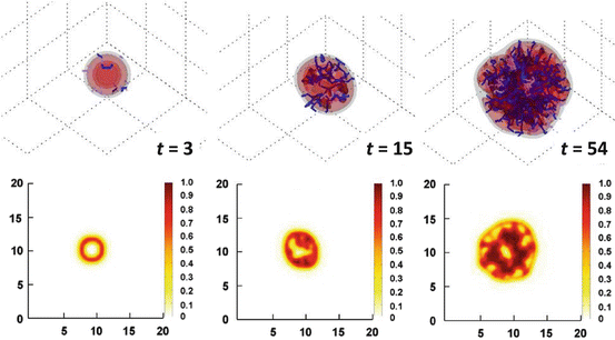

Fig. 2
Simulation of tumor growth in 3D and quantification of tissue density based on vascularization [15]. Upper three panels: A tumor grows uniformly and compactly over time as the surrounding capillary vasculature is stimulated through angiogenesis to supply it with increasing oxygen and nutrient. Tumor invasiveness is lessened compared to the case in Fig. 1, since hypoxic cells are better able to gain access to oxygen and nutrients. Viable tumor tissue (orange/red color) is shown in 3D contours representing density values of 0.1, 0.2, and 0.6 (min.: 0.0; max.: 1.0). Conducting vessels are shown in blue and nonconducting in gray. Time unit = 1 day. Lower three panels: Slices of tumor (plane x = 10) at various times of growth show that viable tumor tissue cuffs around the vessel locations (darker areas), as is typically observed clinically for solid tumors, with areas more distal from the vessels being dead. Color coding: density of viable tissue; highest = 1.0 (unit length = 100 μm). Reprinted with permission from J Theor Biol, Vol. 264, Frieboes et al., Three-dimensional multispecies nonlinear tumor growth-II: Tumor invasion and angiogenesis, pp. 1265–1266, Copyright (2010), with permission from Elsevier
The model predicts that tumor invasiveness depends critically on its coupling with the vasculature. Observations of tumor vasculature function from imaging, when integrated with this type of modeling, could provide further insight into tumor behavior within living patients. Frieboes et al. [15] further simulated the growth of a tumor with one single viable cell species in 3D and included the effects of vessel regression (shutdown) due to the solid (internal tumor) pressure. Figure 3 shows a tumor starting as a small, round avascular nodule at t = 1, which becomes surrounded by new capillaries through the process of angiogenesis (e.g., t = 8 and t = 20). At t ≈ 23 the cell proliferation exerts enough pressure that the blood flow in some of the capillaries becomes impeded, shuts down, and the vascular network regresses. Hypoxia is then locally increased, triggering a higher release of angiogenic factors. The viable cells downgrade their proliferation. Eventually cell homeostasis is disrupted to such an extent that several regions of the tumor undergo necrosis, causing the tumor to regress, thus exacerbating the morphological instability through uneven shrinking of the tumor mass (t = 25). A similar effect has been observed through the model when simulating anti-angiogenic therapy [143], which may shut down the tumor vasculature in an uneven manner and exacerbate tumor break-up and invasion [142, 144–146].
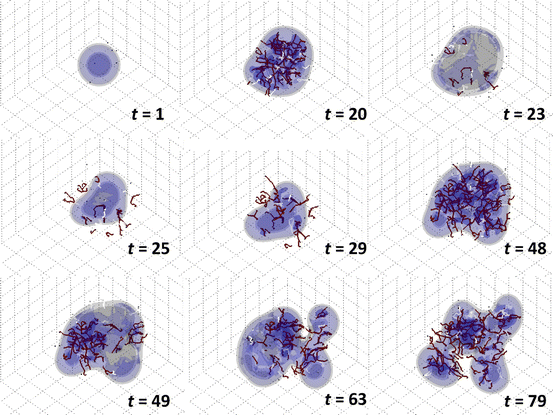

Fig. 3
Simulation of vascularized tumor growth in 3D [15]. Morphological stability of the tumor and its invasiveness are directly linked to the availability of cell substrates regulated by the dynamically evolving vasculature. At time t = 23, the supply of cell substrates is shut off by the collapse of vessels due to increasing pressure from the surrounding proliferating cells. The tumor mass then undergoes temporary regression (t = 25). By t = 29, neovascularization is apparent in response to the increased hypoxia in the interior of the tumor. By t = 48 the tumor has re-grown and is once again highly vascularized. At t = 49 the vessels in the right hemisphere are crushed by the tumor cells. The tumor morphology becomes more unstable, breaking up into two pieces (t = 63). Renewed vascularization eventually helps to restabilize the mass (t = 79). Viable tumor tissue (blue color) is shown in 3D contours representing density values of 0.1, 0.2, and 0.6 (min.: 0.0; max.: 1.0); complete absence of viable tissue is shown in gray. Conducting vessels: brown; nonconducting: white. Time unit = 1 day (grid length = 200 μm). Reprinted with permission from J Theor Biol, Vol. 264, Frieboes et al., Three-dimensional multispecies nonlinear tumor growth-II: Tumor invasion and angiogenesis, pp. 1267–1268, Copyright (2010), with permission from Elsevier
A new round of vessel generation is triggered at t = 25 induced by the production of angiogenic regulators as a result of increased hypoxia in response to continued cell proliferation and tumor necrosis. This second wave of angiogenesis leads to a larger tumor with a more complex morphology than at earlier times, until the pressure from cell proliferation disrupts the blood flow (t = 49) once again. By this time, however, the tumor has gained enough mass so that the disruption predominantly affects the right hemisphere, which leads to tissue break-up in this region. The resulting hypoxia upregulates angiogenesis towards the right side of the tumor, as seen at t = 54. The new vascular network is concentrated more towards the center of the tumor and not at the leading clusters, since these have better access to the surrounding (existing) host vasculature (not shown). By t = 63 vessels become disrupted on the left lobe, which initially shrinks and furthers the splitting of the tumor into two pieces. As cell proliferation once again increases due to enhanced vascularization, the two parts grow larger and begin to reconnect (t = 79). The stability of the tumor morphology and its invasiveness is directly linked to the availability of cell substrates regulated by the evolving vasculature in response to cell proliferation and death.
Stay updated, free articles. Join our Telegram channel

Full access? Get Clinical Tree


