Predicted outcome
Actual outcome
Positive
Negative
Positive
True-positive
False-negative
Negative
False-negative
True-negative
With this concept, we can then calculate the sensitivity and specificity of the technique. The sensitivity is the true-positive rate, and the specificity is the true-negative rate. A ROC curve is a presentation of sensitivity v 1-specificity or false-positive rate. A perfect test will have a 100 % true-positive and true-negative value. A test which has a poor discrimination will have 50 % false results and 50 % true results. This is seen as the line at 45° on the ROC curve. The better a technology or measurement, the closer the curve to the top left corner of the graph. One way two techniques can be compared is to calculate the area under the curve (AUC).
A free web-based application for evaluating ROC curves can be found at: http://www.rad.jhmi.edu/jeng/javarad/roc/JROCFITi.html
However, before we discuss this further, a second differentiation has to be considered: whether the assessment of disease is based on truly quantitative assessments (like a linear measurement, such as joint space narrowing in osteoarthritis or brain volume in Alzheimer’s disease) or a radiological interpretation of an image into a semiquantitative scoring system, like the Genant score for vertebral deformity [5] or Sharp score for rheumatoid arthritis [6].
In general (and this is a generalization, since there are examples that do not follow this distinction), the greater the numerical spread, the “better” the instrument at differentiating between treatments whether it be between active comparators or between active and placebo, particularly for measurement techniques. The definition of normal is different for each therapeutic area. For example, when considering bone densitometry as assessed by dual energy X-ray absorptiometry (DXA), bone ultrasonometry, or quantitative computed tomography (QCT), “normality” is defined by a population of young healthy individuals aged between 20 and 40 without any history of bone disease or medication usage likely to affect bone. The “normal” population should also be drawn from a geographically diverse population to avoid local regional differences. Owing to phenotypic variation, a separate population needs to be assessed for each of the major ethnic groups (e.g., Caucasian, African, and Asian) which has to be further divided by gender. The accepted definition of osteoporosis as defined by the World Health Organization (WHO) is an individual having bone mass less than 2.5 standard deviations (−2.5 SD) below the young normal mean [5]. The definition is also specific to the anatomical area being imaged with different values meeting the criteria for osteoporosis at the hip and at vertebrae. This has come about due to the inverse relationship between DXA measurement and the age-related increase in fracture risk. Once past the menopause there is a decrease in bone mineral density caused by an uncoupling of bone remodeling due to the decrease in circulating estrogens in women. There is a more gradual but age-related loss of bone in men due to the decrease of circulating sex steroids.
By the very definition of the disease being based on a normal population curve, as individuals stay alive they develop age-related bone loss, and a larger percentage of the population will become osteoporotic. However, it is critically important to appreciate that normality is gender, race, and anatomy specific, which creates further challenges when combining populations in clinical trials. However, the concept still remains – the greater the difference between normal and abnormal, the better the overall ability to diagnose with clarity but more importantly in clinical trials, to see a change caused by therapeutic intervention. This is further related to the precision of the measurement which will be discussed further in the next section.
With the so-called semiquantitative measurements, a scaling and graduation scoring system has to be used which is generally a numerical system with 0 being normal or healthy. The common ones are often used in musculoskeletal disease, as already mentioned. The challenge is to have a scoring system which has sufficient granularity to distinguish change by therapeutic intervention or to demonstrate worsening disease without being so complex as to make the scoring system unusable. A great example is the Sharp scoring system, modified by van der Heijde for the evaluation of joint space narrowing and erosions in rheumatoid arthritis [7]. On initial view, it seems very complex, with a total score of 428 (280 for maximum erosion score and 168 for maximum joint space narrowing score), with a score of 0 being a subject with no observable disease radiographically on hands and feet radiographs. However, the score is broken down into a 0–5 (in most instances) for each of 26 joints per hand and feet being evaluated for erosions and again for joint space narrowing, with a slightly different evaluation. On a joint perspective, this makes a relatively simple and reliable scoring technique. Furthermore while there are reader interpretive differences on a per visit basis, these are decreased by evaluating the “change score” between time points. An alternative method that has been used in a number of trials is the Genant score, which has many similarities to the novice evaluator [8]. However the scoring system is reduced to a total of 312 (176 and 136 for maximum erosions and joint space narrowing, respectively). On initial review this would suggest a decrease in sensitivity to detect change, but a potential increase in the reproducibility of the readers to score. There is a subtle twist – the score can be in 0.5 increments! Debate regarding the merits of each scoring system has existed and will continue to do so, and it takes the trialist carefully evaluation as to which is the most pertinent to their trial for other reasons. After all, these scoring systems are not used for routine clinical practice. The final say probably now goes to the regulators; the European Medicines Agency (EMA) has come out with a new guidance for rheumatoid arthritis and stated that the van der Heijde modified Sharp scoring system should be used unless there is a good rational to use another methodology [9].
One further concept has to be considered when evaluating end point in clinical trials: the smallest detectable difference (SDD) or smallest detectable change (SDC). “The SDD expresses the smallest difference between two independently obtained measures that can be interpreted as “real” – that is, a difference greater than the measurement error” [10]. The SDC is a concept that has grown out of the field of rheumatoid arthritis, where there is a dichotomous group of subjects that can be observed in a clinical trial. The majority of subjects show little or no change in the 2 years of observation in their radiological scores, where there is a small subgroup which undergoes a large change in joint damage. Furthermore, since the reads are conducted with a number of time points presented all at one time, the images are not truly independent in the statistical sense. The read design and methodology will be covered more fully in Chap. 5. However, the key difference is that SDD is based on the concept that a patient’s disease is progressing and SDC is based on the concept of how the much less disease is progressing. Either assessment is the determination of the degree of progression above the measurement error that can be statistically determined. In rheumatoid arthritis trials, Bruynesteyn and colleagues conclude that SDD over estimates the number of patients required for the study [10]. SDC has now been used for in other rheumatoid diseases such as ankylosing spondylitis [11]. However, when reviewing the literature using Google Scholar, SDD is the preferred methodological approach in all other therapeutic areas when it comes to radiological interpretations.
Precision and Accuracy
Precision is the term use to describe the reproducibility of the measurement. This is usually assessed by performing multiple repeated measurements using the same measuring instrument on the same patient, for example, measuring a patient’s height or weight on an office scale. It is reported as the percentage coefficient of variation. The lower the %CV, the better the precision and the easier it is to detect small changes in the measurement. To perform true estimates of precision requires the repeat imaging of approximately 20+ subjects or patients. Each image must then be assessed by multiple readers. Due to the ethics of radiation dose for many imaging modalities except perhaps ultrasound and MRI, true precision measurements cannot be acquired. However, repeated measurements of the same images can be performed in order to acquire a reasonable estimate of precision.
Precision is not to be confused with accuracy, which is how close the measurement is to the actual quantity being measured. An example of the difference between precision and accuracy with target shooting is shown in Fig. 2.1. For clinical trials where the measurement is the primary inclusion or exclusion parameter, then the baseline measurement calls for high accuracy. At enrollment, a comparison is made of the individual to a normal reference population to assess the degree of disease. Precision then becomes more important for all future measurements to ensure they compare to baseline. Even if the assessment at baseline was inaccurate, but the patient is included in the study, all future assessments need to be acquired as closely to the baseline measurement – precision is at the cost of accuracy.
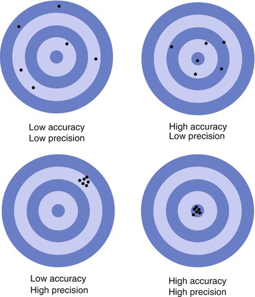
Fig. 2.1
A representation of precision and accuracy using targets
Accuracy is very difficult to assess in many imaging situations. For example, with plain film radiographs there are beam divergence and magnification issues which means there has to be a reference or caliper in the field of view which is of known size. So taking the example of vertebral deformity, a washer or ball bearing should be placed on the skin at the level of a vertebral spinous process (T12 is often used, since it is common to both the lumbar and thoracic lateral spine films). The washer will allow an accurate measure of T12, but at the further proximal or distal column, measurements will be made where there is beam divergence which will create a more significant measurement error, beyond the 4 mm threshold which is usually used to define fracture. This issue is further compounded with patients with significant scoliosis which places the vertebrae higher up the spine in or out of the vertical plane from the caliper and changes the orientation from a true lateral image to a more oblique image for several vertebrae. Accuracy is truly difficult.
MRI is another example where accuracy is difficult to determine field distortion is just one of the issues that occurs. For measurements requiring high precision and accuracy, such as brain or hippocampal volume in Alzheimer’s disease, distortion of the field may create artifactual changes, but which measurement is the most accurate will be unknown until death and biopsy can be used to correlate to the measurements. However, in this Alzheimer’s disease example phantoms should be employed for the trial to monitor and evaluate these changes.
If there are no eligibility criterion requiring imaging, assessment then precision or reproducibility is the overriding parameter to consider. There is an inherent assumption that having selected the use of a particular imaging technique that the manufacturer has ensured that it measures precisely and accurately: this supposition may not be correct. With the sphygmomanometer example earlier, the problem would not have arisen if a calibration check had been performed prior to the start of the study.
Having separately discussed the concepts of precision and in the previous section discrimination, the two parameters cannot be evaluated in isolation. The poorer the discrimination, the higher the precision that is required to distinguish between cohorts or populations. Taking it to the extreme, an instrument with a precision of say 10 % would be of little value if the difference between normal and disease state was only 10 % or even 15 %. With that said, one of the characteristics of clinical trials is the use of groups of subjects to provide a good signal to noise ratio to detect a therapeutic signal amongst the biological noise. Precision has to be factored into the power calculations, which will determine the study size. If the precision, however, is very much less than standard deviation of population mean change, then precision is not the predominating factor. An appreciation for the difference between monitoring a subject’s change to therapy or disease and the group effect of the treatment or disease, where in effect, there is signal averaging to elucidate the change in each treatment group. For example, in the field of osteoporosis, using DXA and the assessment of bone mineral density (BMD) the standard deviation of BMD in a group of subjects will be around 0.1 g·cm−2 with a mean of 1.0 g·cm−2, i.e., about 10 %. The long-term precision of most DXA equipment at the lumbar spine is between 1 and 3 % depending on the study population. While 10 % may not seem significant, this can introduce a large cost burden, so this has to be factored into the study design [12]. Also this example was one where the precision is very much less than the standard deviation of the patient population. If precision is a larger percentage of the SD, e.g., with carotid intima-media thickness (IMT) measurements, then precision has the overriding influence and will significantly drive up patient numbers [13].
A parameter combining dynamic range and precision was developed in the field of bone ultrasonometry, called the standardized coefficient of variation [%SCV] [14]. This is the %CV multiplied by the dynamic range divided by the mean of the measurement. The smaller the %SCV, the better the measurement. Since the measure of precision is affected by the scale being used, it is impossible to compare instruments or imaging techniques using different scales. The %SCV allows for this comparison. Other statistical methodologies have also been proposed [15, 16] to overcome these issues.
Reliability
Reliability has two components: It refers to consistency in the properties of the imaging system (hardware, software, and radiologist or reader) that will provide a reproducible outcome with repeated use and the reliability of the surrogate or imaging biomarker on the end point in the clinical trial. These two aspects will be considered separately.
An imaging technique that cannot be reliability acquired is useless (a liability) in a clinical trial setting. Reliability is the assessment of the change in calibration, however caused. An example of calibration shifts is seen in Fig. 2.2. In this example it is of a DXA instrument calibration, but could be for any other system being assessed over time, e.g., reader calibration and change in MRI inhomogeneities. In this graph each point is a measurement of the same calibration phantom on the DXA scanner. Around September there is a downward shift in the mean calibration of the instrument by an average of 3 %. The calibration remains constant until January where there is an upward shift of 3 % followed by a gradual downward drift in calibration for the remainder of the graph. A subject who is scanned every 6 months starting in May will show a loss of bone mineral density (BMD) of 3 % at the November visit, followed by a nearly increase in BMD of 3 % the following May. After that, the drift is more difficult to characterize, and the effect on the subject BMD is uncertain.
 Radiation Risks and Dosimetry Assessment
 Defining the Radiological Blinded Read and Adjudication
Imaging in Musculoskeletal, Metabolic, Endocrinological, and Pediatric Clinical Trials
Defining the Radiological Blinded Read and Adjudication
Imaging in Musculoskeletal, Metabolic, Endocrinological, and Pediatric Clinical Trials
 Nuclear Medicine: An Overview of Imaging Techniques, Clinical Applications and Trials
 Contrast Agents in Radiology
 Body Composition


Related posts:
Radiation Risks and Dosimetry Assessment
Defining the Radiological Blinded Read and Adjudication
Imaging in Musculoskeletal, Metabolic, Endocrinological, and Pediatric Clinical Trials
Nuclear Medicine: An Overview of Imaging Techniques, Clinical Applications and Trials
Contrast Agents in Radiology
Body Composition
Stay updated, free articles. Join our Telegram channel
Full access? Get Clinical Tree
