The Musical Score
Objectives
At the completion of this chapter, the student should be able to do the following:
• Identify the five lines of a magnetic resonance imaging (MRI) pulse sequence.
• Recognize the various symbols used to diagram an MRI pulse sequence.
• Describe how a slice is selected for imaging.
• Describe how a pixel is located within a slice.
• Relate two ways that slice thickness can be changed.
• Draw the MRI pulse sequence diagrams for partial saturation, inversion recovery, and spin echo.
Key Terms
The magnetic resonance imaging (MRI) system operates like a player piano. The control program for the MRI system is a pulse sequence. The pulse sequence diagram is a complicated schematic containing graphs that show what each major component of the MRI system should be doing at each moment.
The pulse sequence diagram is analogous to the musical score used by a conductor to lead an orchestra. Just as each instrument follows its own line of music in the conductor’s score, each component of the MRI system (i.e., the transmitted radiofrequency [RFt], the received MRI signal [RFs], and the three gradient magnetic fields coils, BSS, BΦ, BR) has its own row of timing information in the pulse sequence diagram.
Fortunately, routine imaging uses preprogrammed pulse sequences, so the MRI technologist needs only to select a programmed technique.
The Purpose of the Pulse Sequences
After the preceding discussions of the physics of MRI and the necessary equipment for MRI, discussion can turn to how magnetic resonance (MR) signals (RFs) make an image and what characterizes the image.
In MRI, a pulse sequence is a set of instructions given to the imaging system to tell it how to make an image. In radiography, instructions are given to the x-ray imaging system by setting the kilovolt peak (kVp) and the milliampere-second (mAs). The manner in which these controls, especially the kilovolt peak control, are positioned influences the contrast of the resulting image.
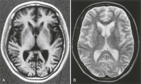
In x-ray imaging, the relative order of the gray scale remains unchanged. Regardless of the kVp, bone always appears brighter than soft tissue. However, with MRI, the relative brightness of different tissues and the contrast rendition can be reversed by changing the timing and magnitude of the radiofrequency (RF) pulses (Figure 14-1).
 The MRI pulse sequence diagram details the timing pattern for the RF pulses and gradient magnetic fields.
In computed tomography (CT), the image time, slice thickness, kVp, field of view, matrix size, and the reconstruction algorithm are selected by the technologist. These choices influence the contrast and spatial resolution of the image.
MRI pulse sequences are analogous to the radiographic and CT selections made by the technologist. The pulse sequences specify the timing and magnitude of the RF pulses and the gradient magnetic fields. The amplitude and timing of the RF pulses affect the image contrast. The pulsed gradient magnetic fields provide spatial localization and influence the spatial resolution of the image.
As in CT, the MR image is formed digitally. In conventional radiography, the image is analog. The MR image is a mosaic of pixels. Each pixel has two properties: character and position. Character refers to the intensity of the pixel.
In a CT image, shades of gray are assigned on the basis of Hounsfield units (HU), which relate to x-ray attenuation values (Figure 14-2). White is assigned to pixels with high attenuation values (e.g., bone); black is assigned to pixels with low attenuation values (e.g., air).
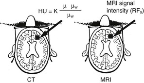
In MRI, the gray scale is assigned on the basis of the intensity of the MR signal emitted from a given voxel (see Figure 14-2). That intensity, in turn, is dependent on the T1, T2, and proton density (PD) of tissue. White is assigned to pixels with high signal intensity; black is assigned to those with low signal intensity. Subsequent chapters fully discuss pixel character and therefore image contrast. This chapter focuses on spatial localization.
 Gradient magnetic fields provide spatial localization of the MR signal (RFs).
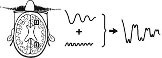
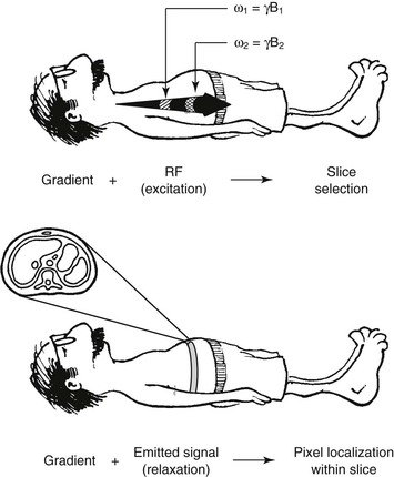
The intensity of the received MR signal (RFs) as it is apportioned among the pixels of the image determines its spatial location. A single signal is emitted from the entire slice after excitation by a slice-selective pulse, (RFt, BSS).
Even though each voxel has its own net magnetization that produces an MR signal, the signal received by the imaging system (RFs) combines the signals from each voxel (Figure 14-3). This differs from radiography, which is basically a projection shadowgram.
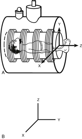
In most MRI systems, the main magnetic field (B0) is horizontal and aligned with the bore of the magnet and the longitudinal axis of the patient. This is true for most superconducting magnets but not for most permanent magnets. In keeping with earlier discussions, a horizontal orientation is assumed for the following discussion.
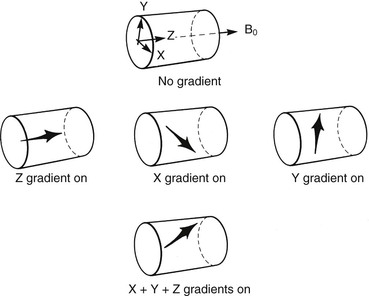
The Z-axis, which is parallel to B0, runs through the center of the magnet in the direction of the long axis of the patient. The X- and Y-axes are perpendicular to Z. X is horizontal and Y is vertical (Figure 14-4).
B0 is intense and is energized throughout the MRI examination. Vendors go to great lengths to ensure that this B0 field is not only intense, but also uniform throughout the imaging volume. Purposefully, the vendors also provide a means of disturbing the field homogeneity systematically and orderly.
This disturbance of field homogeneity is achieved through the use of paired gradient coils. These paired gradient coils are the key features distinguishing an MRI system from a nuclear magnetic resonance (NMR) spectrometer (see Chapter 11).
The gradient coils produce relatively weak magnetic fields superimposed on the B0 field. These gradient coils are intermittently pulsed for milliseconds each time. Each pair of coils produces a small gradient magnetic field along one of the axes.
These small gradient magnetic fields are either parallel or perpendicular to B0. Because the gradient magnetic field varies in intensity along the direction of the axis of the gradient coils, the combined magnetic field is stronger at one end of an axis than at the other.
Gradient Coil Function
The purpose of the gradient magnetic field is twofold: slice selection and pixel localization within the slice. The gradient coils identify which part of the signal belongs in each pixel.
The Larmor equation (ƒ = γB) states that hydrogen nuclei in a magnetic field precess at a frequency (ƒ) that depends on the strength of the magnetic field (B). The constant γ is characteristic of a given nuclear species. For hydrogen, the constant equals 42 MHz/T. If the magnetic field is not homogeneous, protons in a slightly stronger field precess faster than those in a weaker magnetic field (Figure 14-5).
For protons to be excited in an area with a stronger magnetic field, a higher frequency, RFt, is required to match the resonance frequency of those protons. The combination of the magnetic field inhomogeneity produced by the gradient coils and the excitation by a specific RF frequency permits slice selection.
During relaxation, the frequencies of the signals from the protons also depend on the magnetic field strength at the location of each excited proton. When the RFt is turned off and the excited protons relax back to equilibrium, the free induction decay (FID) at the strong end of a gradient magnetic field has higher frequencies than the FID at the weak end of the field. Consequently, the presence of a gradient magnetic field during signal reception helps localize the protons within the slice that was selected during excitation.
Slice Selection
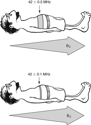
If the Z gradient coils are on, the magnetic field intensity varies linearly from one end of the patient to the other (Figure 14-6). At one end of the magnet, the magnetic field is stronger than at the other end. The proton precessional frequency for a 1 T magnet is 42 MHz. A proton at the strong end may precess at 43 MHz, whereas one at the weak end may precess at 41 MHz.
An RF pulse of exactly 42 MHz excites all of the protons in the plane perpendicular to the Z-axis at the 42-MHz position along the gradient magnetic field. At all other points along the gradient magnetic field, the protons remain unaffected by the 42 MHz RF pulse because they do not resonate at that frequency. They are insensitive to it. In this way, the Z gradient performs slice selection (GSS), and a single transverse slice is selectively excited.
If a gradient along the X-axis were used instead of the Z gradient, the slice selected would be in a sagittal plane. Similarly, a Y gradient would select a coronal plane. In fact, with the X, Y, and Z gradients turned on together, any plane in the body may be chosen (see Figure 14-6). All subsequent discussions assume transverse slice selection; however, the principles apply to slices in any orientation.
The steepness, or slope, of the gradient magnetic field and the range of frequencies, or bandwidth, of the RF pulse determine the thickness of the selected slice. The steeper the gradient magnetic field, the thinner the slice. The narrower the bandwidth of the RF pulse, the thinner the slice.
The purity of an RF pulse is identified by its quality value (Q). The Q of a pulse is the center frequency divided by the bandwidth. As bandwidth becomes more narrow, the Q of an RF pulse becomes higher.
Bandwidth is the range of frequencies contained within the RF pulse (RFt). This is different from the receiver bandwidth, which was discussed in Chapter 13. Ideally we would like to make the RFt arbitrarily small. However, achieving narrow bandwidth comes at a cost. The inverse relationship between time and frequency space is in play for RF pulse production as well as for RF signal sampling. This means that in order to make a slice narrow in thickness the selective RF pulse used must play out for a long time.
 The bandwidth of an RF pulse (RFt) becomes narrower as the duration of the RF pulse is increased.
Long RF pulses cause problems for several reasons. First, the longer the RF pulse then the longer the minimum TE that will be possible for a given pulse sequence. Second, if the RF pulse gets very long then T2 relaxation can cause the signal to decay before the pulse has even ended. We can see that a trade-off must be made so that we have reasonably narrow slice thickness and reasonably short TE values. This explains why the minimum slice thickness available on MRI scanners is rarely less than 3 mm.
In the presence of a fixed Z gradient magnetic field, slice thickness can be selected by changing the bandwidth of the excitation RF pulse (Figure 14-7). Alternatively, slice thickness can be selected by changing the intensity of the gradient magnetic field in the presence of a constant Q RF excitation pulse (Figure 14-8).
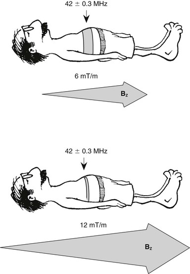
Gradient magnetic field intensity ranges from approximately 10 mT/m to 40 mT/m. The difference is due to the power supply that drives the direct current through the gradient coils. The steeper the applied gradient magnetic field, the thinner the imaged slice.
Usually the frequency width of the RF excitation pulse is fixed for a range of slice thicknesses (e.g., 1 to 10 mm), and the strength of the slice selection gradient magnetic field, BSS, is adjusted to fine-tune the slice thickness within the range allowed by the particular RF excitation pulse.
Pixel Location Within a Slice
Perhaps the most difficult concept to grasp in MRI is how to determine the location of each pixel within a slice. This is because the MR data are acquired in the spatial frequency domain, k-space, whereas radiologists visualize the patient in the spatial domain or pixel position (see Chapter 13).
Related posts:


Stay updated, free articles. Join our Telegram channel

Full access? Get Clinical Tree


