chapter 16 Tomographic Reconstruction in Nuclear Medicine
A basic problem in conventional radionuclide imaging is that the images obtained are two-dimensional (2-D) projections of three-dimensional (3-D) source distributions. Images of structures at one depth in the patient thus are obscured by superimposed images of overlying and underlying structures. One solution is to obtain projection images from different angles around the body (e.g., posterior, anterior, lateral, and oblique views). The person interpreting the images then must sort out the structures from the different views mentally to decide the true 3-D nature of the distribution. This approach is only partially successful; it is difficult to apply to complex distributions with many overlapping structures. Also, deep-lying organs may have overlying structures from all projection angles.
An alternative approach is tomographic imaging. Tomographic images are 2-D representations of structures lying within a selected plane in a 3-D object. Modern computed tomography (CT) techniques, including positron emission tomography (PET), single photon emission tomography (SPECT), and x-ray CT, use detector systems placed or rotated around the object so that many different angular views (also known as projections) of the object are obtained. Mathematical algorithms then are used to reconstruct images of selected planes within the object from these projection data. Reconstruction of images from multiple projections of the detected emissions from radionuclides within the body is known as emission computed tomography (ECT). Reconstruction of images from transmitted emissions from an external source (e.g., an x-ray tube) is known as transmission computed tomography (TCT or, usually, just CT, See Chapter 19, Section B). The mathematical basis is the same for ECT and TCT, although there are obviously differences in details of implementation.
ECT produces images in which the activity from overlying (or adjacent) cross-sectional planes is eliminated from the image. This results in a significant improvement in contrast-to-noise ratio (CNR), as already has been illustrated in Figure 15-11. Another advantage of SPECT and PET over planar nuclear medicine imaging is that they are capable of providing more accurate quantitation of activity at specific locations within the body. This is put to advantage in tracer kinetic studies (Chapter 21).
The mathematics underlying reconstruction tomography was first published by Johann Radon in 1917, but it was not until the 1950s and 1960s that work in radioastronomy and chemistry resulted in practical applications. The development of x-ray CT in the early 1970s initiated application of these principles for image reconstruction in medical imaging. An interesting historical perspective on the origins and development of tomographic image reconstruction techniques is presented in reference 1.
Instrumentation for SPECT imaging is discussed in Chapter 17 and instrumentation for PET is discussed in Chapter 18. Although the instruments differ, the same mathematics can be used to reconstruct SPECT or PET images. In this chapter, we focus on the basic principles of reconstructing tomographic images from multiple projections. A detailed mathematical treatment of image reconstruction is beyond the scope of this text. The reader is referred to references 2 to 4 for more detailed accounts.
a General Concepts, Notation, and Terminology
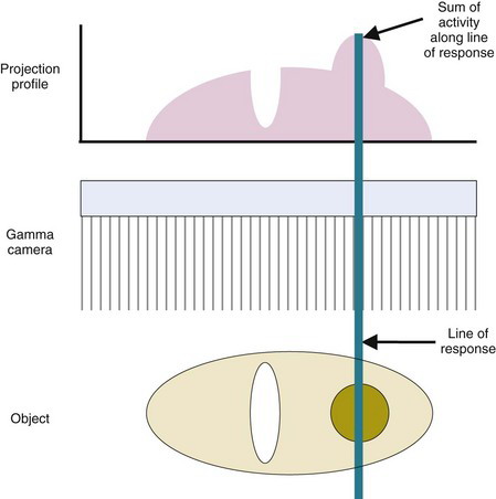
We assume initially that data are collected with a standard gamma camera fitted with a conventional parallel-hole collimator. (Applications involving other types of collimators are discussed in Section E.) To simplify the analysis, several assumptions are made. We consider only a narrow cross-section across the detector. The collimated detector is assumed to accept radiation only from a thin slice directly perpendicular to the face of the detector. This reduces the analysis to that of a 1-D detector, as shown in Figure 16-1. Each collimator hole is assumed to accept radiation only from a narrow cylinder defined by the geometric extension of the hole in front of the collimator. This cylinder defines the line of response for the collimator hole. For further simplification, we ignore the effects of attenuation and scatter and assume that the counts recorded for each collimator hole are proportional to the total radioactivity contained within its line of response. The measured quantity (in this case, counts recorded or radioactive content) sometimes is referred to as the line integral for the line of response. A full set of line integrals recorded across the detector is called a projection, or a projection profile, as illustrated in Figure 16-1.
Obviously, the assumptions noted earlier are not totally valid. Some of the effects of the inaccuracies of these assumptions are discussed in Chapter 17, Section B and in Chapter 18, Section D.
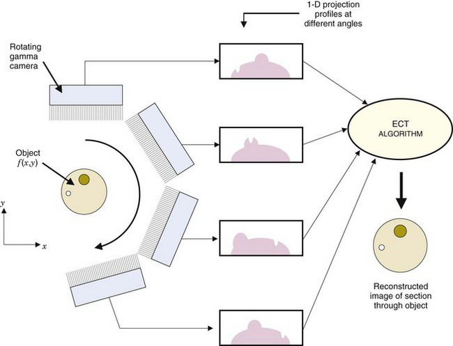
A typical SPECT camera is mounted on a gantry so that the detector can record projections from many angles around the body. PET systems generally use stationary arrays of detector elements arranged in a ring or hexagonal pattern around the body. In either case, the detectors acquire a set of projections at equally spaced angular intervals. In reconstruction tomography, mathematical algorithms are used to relate the projection data to the 2-D distribution of activity within the projected slice. A schematic illustration of the data acquisition process is shown in Figure 16-2. Note that the data collected correspond to a slice through the object perpendicular to the bed and that this is called the transverse or transaxial direction. The direction along the axis of the bed, which defines the location of the slice, is known as the axial direction.
We assume that N projections are recorded at equally spaced angles between 0 and 180 degrees. Under the idealized conditions assumed here, the projection profile recorded at a rotation angle of (180 + φ) degrees would be the same (apart from a left-right reversal) as the profile recorded at φ degrees. Thus the data recorded between 180 and 360 degrees would be redundant; however, for practical reasons (e.g., attenuation), SPECT data often are acquired for a full 360-degree rotation. This is discussed further in Chapter 17.
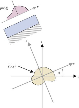
For purposes of analysis, it is convenient to introduce a new coordinate system that is stationary with respect to the gamma camera detector. This is denoted as the (r,s) coordinate system and is illustrated in Figure 16-3. If the camera is rotated by an angle φ with respect to the (x,y) coordinate system of the scanned object, the equations for transformation from (x,y) to (r,s) coordinates can be derived from the principle of similar triangles and are given by
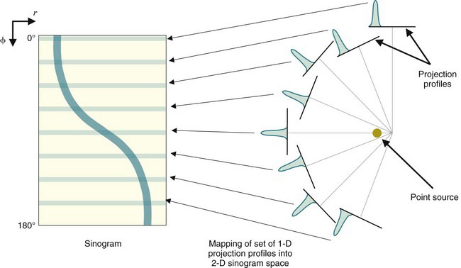
One commonly used way to display a full set of projection data is in the form of a 2-D matrix p(r,φ). A representation of this matrix, generically known as a sinogram, is shown for a simple point-source object in Figure 16-4. Each row across the matrix represents an intensity display across a single projection. The successive rows from top to bottom represent successive projection angles. The name sinogram arises from the fact that the path of a point object located at a specific (x,y) location in the object traces out a sinusoidal path down the matrix. (This also can be deduced from Equations 16-1 and 16-2.) The sinogram provides a convenient way to represent the full set of data acquired during a scan and can be useful for determining the causes of artifacts in SPECT or PET images.
b Backprojection and Fourier-Based Techniques
1 Simple Backprojection
The general goal of reconstruction tomography is to generate a 2-D cross-sectional image of activity from a slice within the object, f (x,y), using the sinogram, or set of projection profiles, obtained for that slice. In practice, a set of projection profiles, p(r,φi), is acquired at discrete angles, φi, and each profile is sampled at discrete intervals along r. The image is reconstructed on a 2-D matrix of discrete pixels in the (x,y) coordinate system. For mathematical convenience, the image matrix size usually is a power of 2 (e.g., 64 × 64 or 128 × 128 pixels). Pixel dimensions Δ x and Δy can be defined somewhat arbitrarily, but usually they are related to the number of profiles recorded and the width of the sampling interval along r.
The most basic approach for reconstructing an image from the profiles is by simple backprojection. The concepts will be illustrated for a point source object. Figure 16-5A shows projection profiles acquired from different angles around the source. An approximation for the source distribution within the plane is obtained by projecting (or distributing) the data from each element in a profile back across the entire image grid (Fig. 16-5B). The counts recorded in a particular projection profile element are divided uniformly amongst the pixels that fall within its projection path.* This operation is called backprojection. When the backprojections for all profiles are added together, an approximation of the distribution of radioactivity within the scanned slice is obtained. Mathematically, the backprojection of N profiles is described by
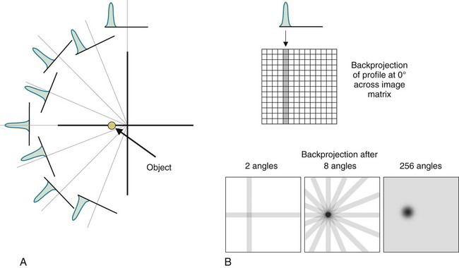
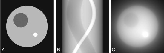
As illustrated in Figure 16-5B, the image built up by simple backprojection resembles the true source distribution. However, there is an obvious artifact in that counts inevitably are projected outside the true location of the object, resulting in a blurring of its image. The quality of the image can be improved by increasing the number of projection angles and the number of samples along the profile. This suppresses the “spokelike” appearance of the image but, even with an infinite number of views, the final image still is blurred. No matter how finely the data are sampled, simple backprojection always results in some apparent activity outside the true location for the point source. Figure 16-6 shows an image reconstructed by simple backprojection for a somewhat more complex object and more clearly illustrates the blurring effect.
Mathematically, the relationship between the true image and the image reconstructed by simple backprojection is described by
where the symbol * represents the process of convolution described in Appendix G. A profile taken through the reconstructed image for a point source that is reconstructed from finely sampled data decreases in proportion to (1/r), in which r is the distance from the center of the point-source location. Because of this behavior, the effect is known as 1/r blurring. Simple backprojection is potentially useful only for very simple situations involving isolated objects of very high contrast relative to surrounding tissues, such as a tumor with avid uptake of a radiopharmaceutical that in turn has very low uptake in normal tissues. For more complicated objects, more sophisticated reconstruction techniques are required.
2 Direct Fourier Transform Reconstruction
Basic concepts of FTs are discussed in Appendix F. Briefly, in the context of nuclear medicine imaging, the FT is an alternative method for representing spatially varying data. For example, instead of representing a 1-D image profile as a spatially varying function, f (x), the profile is represented as a summation of sine and cosine functions of different spatial frequencies, k. The amplitudes for different spatial frequencies are represented in the FT of f (x), which is denoted by F(k). The operation of computing the FT is symbolized by
FTs can be calculated quickly and conveniently on personal computers, and many image and signal-processing software packages contain FT routines. The reader is referred to Appendix F for additional information about FTs.
The concept of k-space will be familiar to readers who have studied magnetic resonance imaging (MRI), because this is the coordinate system in which MRI data are acquired. To reconstruct an image from its 2-D FT, the full 2-D set of k-space data must be available (Equation 16-7). In MRI, data are acquired point-by-point for different (kx, ky) locations in a process known as “scanning in k-space.” There is no immediately obvious way to directly acquire k-space data in nuclear medicine imaging. Instead, nuclear medicine CT relies on the projection slice theorem, or Fourier slice theorem. In words, this theorem says that the FT of the projection of a 2-D object along a projection angle φ [in other words, the FT of a profile, p(r,φ)], is equal to the value of the FT of the object measured through the origin and along the same angle, φ, in k-space (note, the value of the FT, not the projection of the FT). Figure 16-7 illustrates this concept. Mathematically, the general expression for the projection slice theorem is
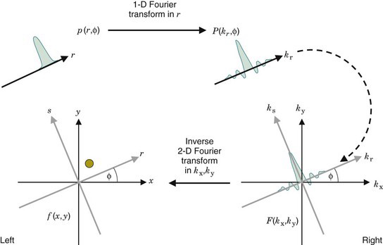
The projection slice theorem provides a means for obtaining 2-D k-space data for an object from a series of 1-D measurements in object space. Figure 16-7 and Equation 16-8 provide the basis for reconstructing an object from its projection profiles as follows:
where primed notation is used to indicate that the coordinate locations do not correspond exactly to points on a rectangular grid. The inserted values are closely spaced near the origin and more widely spaced farther away from the origin. This “over-representation” of data near the origin in k-space is one explanation for the 1/r blurring that occurs in simple backprojection, as was discussed in Section B.1.
3 Filtered Backprojection
Step 5 is essentially the same as simple backprojection, but with filtered profiles. However, unlike Equation 16-3, in which f′ (x,y) is only an approximation of the true distribution, FBP, when applied with perfectly measured noise-free data, yields the exact value of the true distribution, f (x,y). Figure 16-9 schematically illustrates the process of FBP for a pointlike object.
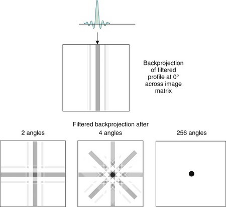
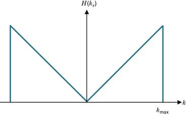
The only difference between simple and filtered backprojection is that in the latter method, the profiles are modified by a reconstruction filter applied in k-space before they are backprojected across the image. The effect of the ramp filter is to enhance high spatial frequencies (large kr) and to suppress low spatial frequencies (small kr). The result of the filtering is to eliminate 1/r blurring.* One way to visualize the effect is to note that, unlike unfiltered profiles (see Fig. 16-5), the filtered profiles have both positive and negative values (see Fig. 16-9). The negative portions of the filtered profiles near the central peak “subtract out” some of the projected intensity next to the peak that otherwise would create 1/r blurring.
Amplification of high spatial frequencies in FBP also leads to amplification of high-frequency noise. Because there usually is little signal in the very highest frequencies of a nuclear medicine image, whereas statistical noise is “white noise” with no preferred frequency, this also leads to degradation of signal-to-noise ratio (SNR). For this reason, images reconstructed by FBP appear noisier than images reconstructed by simple backprojection. (This is a general result of any image filtering process that enhances high frequencies to “sharpen” images.) In addition, filters that enhance high frequencies sometimes have edge-sharpening effects that lead to “ringing” at sharp edges. This is an unwanted byproduct of the positive-negative oscillations introduced by the filter, illustrated in the filtered profile at the top of Figure 16-9.
To minimize these effects on SNR and artifacts at sharp edges, the ramp filter usually is modified so as to have a rounded shape to somewhat suppress the enhancement of high spatial frequencies. Figure 16-10

Stay updated, free articles. Join our Telegram channel

Full access? Get Clinical Tree


