(12.1)
In addition, spectral resolution is expected to improve since the frequency difference (chemical shift, σ) between different metabolites (measured in Hz) also increases linearly
(12.2)
However, some factors adversely affect SNR and resolution as field strength increases, in particular in vivo T 2 and T 2* relaxation times are shorter, and in fact an almost linear increase in metabolite line widths (=1/T 2*) occurs with increasing field strength [12, 13]. The decrease in metabolite T 2 was considered “anomalous” when first observed, as “classically” in MR spectroscopy, T 2 is expected to not change with resonance frequency [2]. However, both metabolite T 2 (as measured using single-echo, rather than Carr-Purcell-Meiboom-Gill (CPMG) sequences) and T 2* relaxation times in brain are shortened by the presence of paramagnetic deoxyhemoglobin in the brain’s microvasculature (a microscopic susceptibility effect) which causes field-dependent linewidth increases [14]. Therefore, while spectral quality at 3 T is superior to that at 1.5 T, improvements in both SNR and spectral resolution are somewhat less than predicted by simple theoretical considerations [8, 15]. For instance, one study found a 28 % improvement in SNR for NAA in short TE spectra, less than the “simple” prediction of 100 % [8]. Since for compounds such as N-acetyl aspartate (NAA), choline (Cho), or creatine (Cr) the improvements in SNR are quite small, it is perhaps not surprising that studies based on these resonances did not find any improvement in “diagnostic quality” at 3.0 T compared to 1.5 T [16]. However, probably the biggest improvements at higher field strengths are for metabolites which are “harder to detect,” i.e., those with relatively lower signal intensities and those which overlap with signals from other compounds—some examples include γ-aminobutyric acid (GABA), glutamate (Glu), and glutamine (Gln). Figure 12.1 shows representative spectra from normal human brain at 1.5, 3.0, and 7.0 T, recorded under similar (but not identical) conditions. It can be seen that the 7 T spectrum shows the best SNR, and that the fine detail in the regions of the spectra containing Glu, Gln, and other resonances (e.g. 2.1–2.6 ppm, 3.5–3.9 ppm) has greater fine detail at 7 T. Figure 12.2 shows simulations of Glu and Gln as a function of field strength ranging from 1.5 to 9.4 T—it can be seen at 1.5 T there is almost complete overlap of the C3 and C4 multiplets of Glu and Gln, but that as the field strength increases the C4 resonances start to separate, and that by 7 T there is almost complete separation of the two.
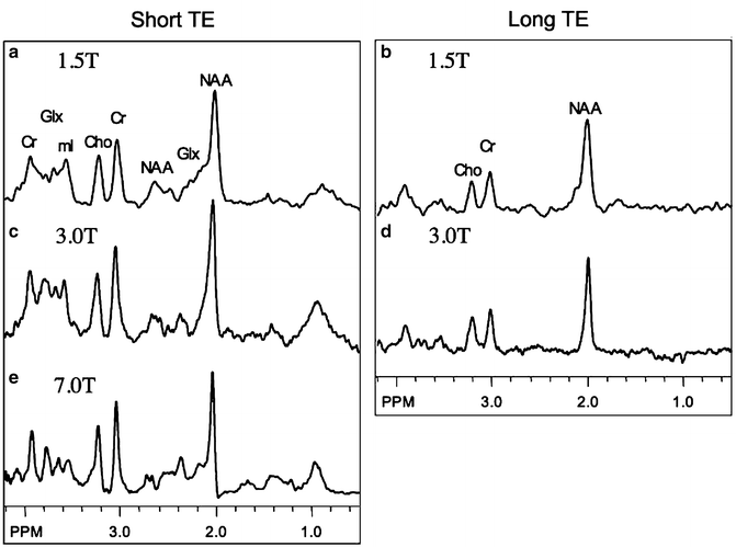
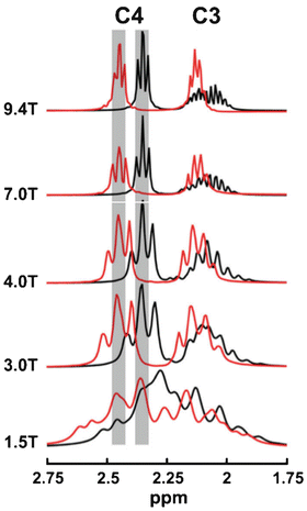
Fig. 12.1
Representative spectra at short (~35 ms) and long (~280 ms) TE from centrum semiovale white matter at 1.5 T (a, b), 3.0 T (c, d), and 7.0 T (e). (a–d) are taken from [8], (e) courtesy of Dr Murdoch
Fig. 12.2
Simulations of the C4 and C3 proton resonances of glutamate (Glu) and glutamine (Gln) as a function of field strength ranging from 1.5 to 9.4 T. The C2 protons which resonate around ~3.75 ppm are not shown. It can be seen that the C4 protons of Glu and Gln become increasingly well resolved with increasing field strength. Adapted with permission from [56]
The fair comparison of spectra between different field strengths is a difficult undertaking, as it is quite rare for MR systems to be “identical” other than the strength of the magnetic field. For instance, similar RF coils, preamplifiers, and receiver electronics, as well as pulse sequences, slice selective pulses, and data processing methods should be used at both field strengths. Indeed, a “philosophical” question is whether identical methods should be in fact be used at both field strengths, or whether different (i.e., optimal) methods are used at each field strength.
Relatively few studies have systematically compared 7 T MRS to lower fields [12, 13, 17]. One study compared 3 and 7 T MRS using very similar methodology at both field strengths, including the use of the same pulse sequence (very short echo time (TE—6 ms) “SPECIAL,” see below) and quadrature transmit-receive surface coils which provided coverage of posterior brain regions [17]. This study found an increased sensitivity by a factor of 1.7 (per unit time) at 7 T compared to 3 T, and improved accuracy of determination for 12 different metabolites. Figure 12.3 shows an example of 3 and 7 T spectra from the anterior cingulate cortex recorded with 32-channel head coils using the semi-LASER (sLASER, see below) in the same subject; while the spectra look quite similar on initial inspection, the 7 T spectra have about a 48 % improvement in SNR compared to 3 T in this example.
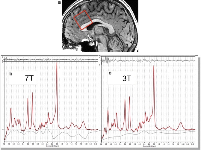
Fig. 12.3
(a) Sagittal MRI showing the 3 × 3 × 3 cm voxel location in the anterior cingulate cortex (ACC) in one subject scanned under identical conditions at both (b) 7 T and (c) 3 T, using 32-channel head coils and the sLASER pulse sequence. Scan parameters were TR/TE 3,000/32 ms, 32 averages, 1 min 36 s scan time. Average SNR in four subjects was 50.1 at 7 T and 33.8 at 3 T (i.e., 48 % improvement at 7 T). Spectral line widths were 0.030 ppm (8.9 Hz) at 7 T and 0.035 ppm (4.5 Hz) at 3 T. Spectra are fit using LCModel software (red line—fit results, gray line estimated spectral baseline, and the top trace is the difference between the experimental data and the fit)
Pulse Sequences for High-Field MRS
General Considerations
As already mentioned above, magnetic susceptibility effects (both microscopic and macroscopic) increase linearly with increasing magnetic field strength. Therefore, in order to achieve expected improvements in spectral resolution, it is important that the magnetic field homogeneity is fully optimized at high-field strengths. Automated shimming routines using field maps and high-order shim (second and third) corrections have been shown to give the best results [18, 19] provided that strong enough shim currents are available.
Radiofrequency (RF) coil design is also important for studies at high field. RF head coils that give uniform B 1 fields at 1.5 or 3.0 T (such as “birdcage” or other resonator coils [20]) have appreciable inhomogeneities at 7.0 T [21], which can result in significant spatial variations in image intensity and contrast, and in the context of MRS, can result in reduced sensitivity, suboptimal water or lipid suppression, or quantification errors. This may particularly be a problem if the scanner flip angle optimization routine is performed on a different (and/or larger) volume than the localized MRS experiment; therefore it is important to make sure that the flip angle is correctly optimized on a volume that closely matches the MRS region of interest [22].
There is also currently interest in multiple coil/amplifier systems to overcome the problem of transmit B 1 inhomogeneity [23, 24]; also, as discussed below, it is possible to use pulse sequence design to minimize the effects of these transmit B 1 inhomogeneities. Similar to lower field strengths, best SNR is obtained (both for MRI and MRS) using multiple, phased-array receiver coils with optimal channel combination [25].
Single Voxel (SV) MRS
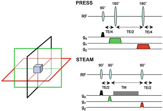
Similar pulse sequences as used at 1.5 or 3.0 T can also be used for 7.0 T, such as the commonly used STEAM [6] or PRESS [26] sequences (Fig. 12.4). However, results may not always be optimal if directly using a 1.5 or 3.0 T protocol at 7.0 T. Various issues may arise: first of all, use of long echo times (e.g., TE 140 or 280 ms) is generally not advised because of the shorter metabolite T 2s at higher field. In addition, the sequence should be designed to be as insensitive as possible to variations in the transmit B 1 field, and, in addition, slice selective RF pulses should be used with high bandwidths in order to minimize “chemical shift displacement” CSD effects [27]. The magnitude of the CSD is given by
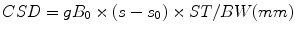
where ST is the slice thickness in mm, BW is the bandwidth of the slice selective pulse (Hz), and σ 0 is the chemical shift corresponding to the scanner transmitter (“center”) frequency (usually the water chemical shift (4.7 ppm) for MRI, but for MRS should be applied in the middle of the spectral region of interest (e.g., ~2.5 ppm if desired to cover metabolites from ~4 to ~1 ppm)). For instance, if the RF pulse has a bandwidth of 430 Hz, for a 15 mm slice thickness the CSD is 10.4 mm/ppm, since 1 ppm = 298 Hz at 7 T. Therefore, in this example, the resonances of myo-inositol (mI at 3.56 ppm) and NAA (2.02 ppm) in the spectrum will originate from totally different slice locations (1.56 ppm ≡16.2 mm, i.e., more than 1 slice thickness) (Fig. 12.5). Solutions to this problem include using higher transmit B 1 fields to increase the pulse bandwidth, or using alternative RF pulse waveforms with higher bandwidths. Figure 12.6a shows an example of a frequency modulated 90° excitation pulse [28] which has a duration of 8.7 ms, maximum amplitude of 13.5 μT, and a bandwidth of 4.7 kHz. Use of such a high bandwidth pulse minimizes the chemical shift dispersion problem (the mI-NAA displacement drops to ~10 % of the slice thickness (Fig. 12.6b)). However, these pulses are typically longer and require more RF power than lower bandwidth pulses, thereby increasing the SAR of the sequence. SAR is a significant concern for high-field MRS, since the SAR is predicted to increase with approximately the square of the Larmor frequency (ω 0 = γB 0) [21].
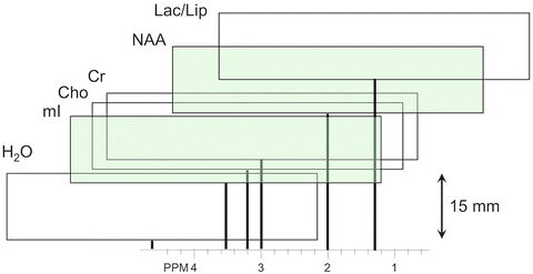
Fig. 12.4
Schematic illustration (note; not all gradients shown, graphic illustration only) of conventional pulse sequences for single voxel MRS; STEAM and PRESS. Both sequences involve the application of three slice selective pulses with field gradients applied in orthogonal directions
(12.3)
Fig. 12.5
Graphic illustration of the chemical shift displacement effect; the slice location for each metabolite is displayed as a function of its chemical shift. Slice locations are displayed for a 15 mm thick slice at 7 T (298 Hz/ppm) for a slice selective pulse with a bandwidth of 430 Hz (≈10 μT). It can be seen the resonances of mI and NAA (shaded green) originate from entirely different (non-overlapping) slice locations (mI-NAA CSD = 1.54 ppm = 458 Hz, CSD = 458/430 = 106 %)
Fig. 12.6
(a) An example of a high bandwidth amplitude and frequency modulated excitation pulse (“fremex05,” courtesy of Dr James Murdoch, [57]) with a duration of 8.7 ms, a maximum B 1 amplitude of 13.5, and a frequency-sweep (bandwidth) of 4.7 kHz. The pulse has been numerically optimized to give a rectangular excitation profile and uniform flip angle over a range of B 1 values. (b) Illustration of the large reduction (compared to Fig. 12.5) of the chemical shift displacement artifact at 7 T using this pulse; with a bandwidth of 4.7 kHz, the mI-NAA CSD is now only ≈10 % (1.5 mm for a 15 mm slice thickness)
While frequency modulated pulses can be incorporated into sequences such as PRESS and STEAM, their increased duration limits the shortest echo times (TE) that can be used. STEAM is arguably favorable to PRESS at high fields in that 90° pulses are somewhat easier to design than 180° pulses, in terms of bandwidth, slice profile and SAR, and relatively short TEs can be obtain (due to the TM time period during which the magnetization is on the Z-axis). However, STEAM only detects the stimulated echo created by the three 90° pulses, which has half of the full signal magnitude. Therefore an alternative approach, dubbed “SPECIAL” [17], was designed to detect the full signal while still maintaining short TE, but using a slice selective inversion pulse (turned on and off on alternating scans) to achieve spatial localization in one direction (Fig. 12.7). SPECIAL works well, but does have the potential for subtraction artifacts since it is a localization method based on subtracting two scans. SPECIAL can be implemented with a frequency swept adiabatic inversion pulse, not only providing a high bandwidth but also to provide full inversion even in the presence of an inhomogeneous transmit field (provided that the minimum transmit B 1 is above the “adiabatic threshold” of the pulse used).
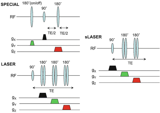
Fig. 12.7
Alternative pulse sequences for SV MRS which may be preferable at high magnetic field strengths: SPECIAL, LASER, and semi-LASER (sLASER). All three sequences make use of adiabatic RF pulses; only LASER is fully adiabatic, however
Pulse sequences may be made fully adiabatic (i.e., theoretically giving the full signal, even if the transmit B 1 is inhomogeneous, or not properly calibrated) by replacing all the pulses in the sequence with adiabatic pulses [29]; this type of sequence was dubbed “LASER” [30]; since frequency swept adiabatic pulses induce a strong, frequency-dependent phase error when used as refocusing pulses, they have to be used in pairs (the phase error of the second pulse reverses (i.e., cancels out) the phase error associated with the first). The LASER sequence is fully adiabatic, but does have quite a long minimum TE because six adiabatic 180° pulses are required, in addition to a non-slice selective adiabatic 90° excitation pulse (Fig. 12.7); because of the 7 RF pulses, the SAR of the sequence is also quite high. A “compromise” sequence that has become quite popular at high fields (e.g., 3 and 7 T) is the “semi-LASER” (sLASER) sequence which retains a non-adiabatic slice selective excitation pulse and uses two pairs of adiabatic refocusing pulses [31, 32] (Fig. 12.7). This sequence is adiabatic in two dimensions, with a somewhat shorter minimum TE and lower SAR than the full LASER sequence. Figure 12.3 shows example spectra from the human brain (anterior cingulate gyrus) recorded at 3 and 7 T user the sLASER sequence. Because of the higher spectral resolution and signal-to-noise ratios available at 7 T, more compounds can be accurately determined compared to lower field strengths; using the “LCModel” analysis method, it has been shown that up to 17 compounds can be estimated [13]. Figure 12.8 shows reproducibility for 7 T STEAM MRS anterior cingulate data from five subjects; in this study, the average coefficient of variation was ~6 %, and in addition to the reliable determination of compounds readily detected at lower fields (tNAA, tCt, tCho, Glx, and mI) it is noteworthy that reliable estimates of glutamate (Glu), glutamine (Gn), γ-aminobutyric acid (GABA), and N-acetylaspartyl glutamate (NAAG) are obtained, among others.
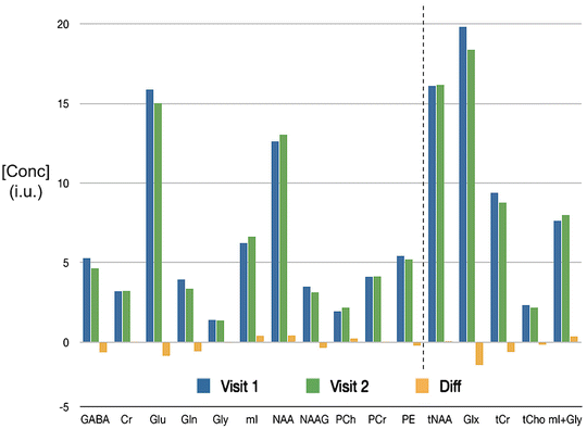
Fig. 12.8
An example of a 7 T MRS reproducibility study; short TE STEAM spectra recorded at 7 T from the anterior cingulate cortex were analyzed with LCModel software to yield concentration values (institutional units—i.u.). Metabolite concentrations (N = 5) are shown for 11 different compounds (and the composite signals tNAA (NAAG + NAA), Glx (Glu + Gln), tCr (Cr + PCr), tCho (PCh + PE), (mI + Gly)) recorded in the same subjects 1 week apart. The average coefficient of variation (CV) was approximately 6 %. Data from [58]
All SV-MRS sequences are generally also performed with water suppression pulses, some of which are optimized specifically for use at 7 T [33]; also, outer-volume suppression (OVS) [34] and phase-cycling [35] are typically used to remove residual signals from outside the target region of interest. Frequency-selective lipid suppression may also be applied [27], particular in conjunction with MR spectroscopic imaging (MRSI) sequences (see below).
MRSI
A wide variety of methods exist for MRSI [36]. MRSI may be performed in one, two, or three spatial dimensions and combined with many of the sequences mentioned above to limit the spatial extent of excitation. A commonly used MRSI sequence at 1.5 or 3.0 T in clinical applications is the 2D-PRESS-MRSI sequence [37], which combines PRESS excitation (limited to one-slice) with two-dimensional phase-encoding. The PRESS volume is chosen to excite as much of the slice as possible while at the same time avoiding exciting the subcutaneous lipid signals in the scalp. The PRESS sequence can also be used with a thicker slice and 3D phase-encoding (3D-PRESS-MRSI) to extend coverage to three dimensions. While 3D-PRESS-MRSI has been demonstrated at 7 T [38], it does have appreciable problems. First, coverage is incomplete because the rectangular PRESS voxel cannot be placed close to the surface of the brain without also including lipids. In addition, voxels near the edges cannot be reliably interpreted because of the pulse profile of the slice selective pulses (particularly the 180° pulses) and chemical shift dispersion effects. If a STEAM sequence is used, the slice profiles are somewhat better since all the slices are defined by 90° pulses, and SAR is also lower; however, SNR will be lower than in PRESS (as discussed above, STEAM has about 50 % of the signal compared to PRESS).
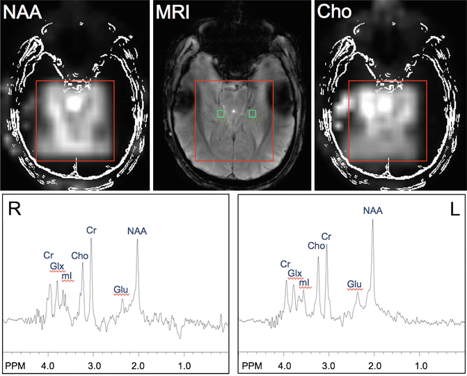
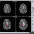
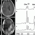
Figure 12.9 shows an example of a 2D-STEAM-MRSI scan of a patient with right-sided mesial temporal lobe epilepsy recorded at 7 T. It can be seen that the body of the right hippocampal body has a lower ratio of NAA/Cho and NAA/Cr than the left, in spite of the fact that the conventional MRI was considered normal in this case.
Get Clinical Tree app for offline access
Fig. 12.9
An example of a 7 T 2D-MRSI scan performed using STEAM localization in a patient with seizures of right
 Imaging Metabolic and Molecular Functions in Brain Tumors with Positron Emission Tomography (PET)
 BOLD fMRI for Presurgical Planning: Part II
 BOLD fMRI for Presurgical Planning: Part I
 Role of Amide Proton Transfer (APT)-MRI of Endogenous Proteins and Peptides in Brain Tumor Imaging
 Future Clinical Applications of Molecular Imaging: Nanoparticles, Cellular Probes, and Imaging of Gene Expression
 Proton Magnetic Resonance Spectroscopy and Spectroscopic Imaging of Primary Brain Tumors


Related posts:
Imaging Metabolic and Molecular Functions in Brain Tumors with Positron Emission Tomography (PET)
BOLD fMRI for Presurgical Planning: Part II
BOLD fMRI for Presurgical Planning: Part I
Role of Amide Proton Transfer (APT)-MRI of Endogenous Proteins and Peptides in Brain Tumor Imaging
Future Clinical Applications of Molecular Imaging: Nanoparticles, Cellular Probes, and Imaging of Gene Expression
Proton Magnetic Resonance Spectroscopy and Spectroscopic Imaging of Primary Brain Tumors
Stay updated, free articles. Join our Telegram channel
Full access? Get Clinical Tree
