7 Projection X-ray imaging offers two-dimensional imaging of a body part of interest. To this day, projection X-ray imaging remains the mainstay of medical imaging, as in many applications, such two-dimensional “compression” of three-dimensional structure is most efficient to characterize the health state of the patient. However, in many other applications, increasingly, the two-dimensional projections are insufficient. The three-dimensional structure can overlap one another, masking relevant information or complicating the interpretation process. For example, in a conventional radiograph, objects with a subtle contrast (less than about 5%) can be obscured from view by the structured anatomic noise created when a 3D anatomy is projected onto a 2D radiographic image plane. For such applications, it is possible to acquire X-ray images volumetrically. Currently, there are two volumetric X-ray imaging methods in use, tomosynthesis and computed tomography (CT). They both exploit radiographic projection process and technology to form three-dimensional, volumetric images. CT in particular has become ubiquitous in medical imaging. It offers the ability to resolve individual slices through a subject, free from overlying anatomic noise. This is what makes CT a powerful imaging modality. However, CT requires expensive dedicated hardware and generally higher radiation dose to the patient than an X-ray radiograph. Therefore, it is unrealistic to replace all of projection X-ray imaging with CT. Tomosynthesis, building upon radiography technology, offers an alternative of using limited projection angles and dose to add three dimensionality to projection images, but not to the extent, dose, and expense of CT. Tomosynthesis is a quasi-3D imaging technology that fills the large void between purely 2D radiography and fully 3D CT. It can be implemented easily on modern digital radiographic X-ray imaging systems, removing the need for expensive CT hardware, and requires an imaging dose only slightly greater than that of a radiograph, all while acquiring a set of cross-sectional images that are largely free of confounding overlying anatomy from distant planes. Spurred by the increasing availability of a new generation of digital flat panel X-ray detectors, the past decade has witnessed the commercial release and increasing adoption of tomosynthesis imaging for a variety of diagnostic imaging tasks, along with a great deal of research into its applications for other medical uses such as patient positioning before conformal radiotherapy. The most common applications today include breast imaging, chest imaging, and musculoskeletal imaging. To demonstrate the difference between tomosynthesis and planar radiography, a chest radiograph and coronal midlung tomosynthesis slice are shown side by side in Figure 7.1. Figure 7.1 Sample posterior–anterior (PA) radiograph (a) and coronal midlung tomosynthesis plane (b) of a human chest subject, acquired with a 20° scan angle. Source: Godfrey et al. 2013 [1]. Reproduced with permission of John Wiley & Sons. Tomosynthesis technology uses an apparatus very similar to that of projection X-ray imaging, with the additional ability of angulation of the beam around the body part of interest and a dynamic detector able to capture multiple images sequentially from each angle projection. An antiscatter grid is conventionally used, as in projection imaging, to minimize the scatter contribution to the image, with the direction of beam angulation chosen to minimize the grid cutoff (see Chapter 6). The projection images are reconstructed to form the three-dimensional tomosynthesis dataset. Long before CT was invented, there existed conventional tomography, which was a simple radiographic imaging method that allowed radiologists to minimize the visibility of overlying structures. Only two decades after Wilhelm Röntgen’s discovery of X-rays in 1895, Johann Radon released a paper in 1917 describing how projection data from different angles could be used to solve for the location of detail deep within the body, which incidentally laid the foundation for the later development of fully 3D CT, magnetic resonance imaging, etc. Following Radon’s contribution, Dutch researcher Ziedses des Plantes introduced the concept of “geometric” or “conventional” tomography in 1932, and UK radiologist Ernest Twining carried it to clinical prominence. In the conventional (twining) tomography geometry (Figure 7.2), an X-ray tube and image receptor are coupled such that they pivot about a fulcrum point, while remaining pointed at one another. This fulcrum point is adjusted to match the depth of interest in a patient, and then the tube and receptor are moved in a continuous sweep while the tube produces a constant X-ray flux such that the receptor integrates the signal received throughout the entire sweep. Because of the principle of parallax, an object at the depth of the fulcrum point appears stationary in the integrated image, while the shadow of an object outside that plane appears to move across the image receptor during the sweep such that the distance of movement increases with the object’s distance from the fulcrum plane. When all of these images are summed together, detail in the fulcrum plane reinforces itself to yield full resolution and signal strength, whereas detail from distant planes is blurred so that their contribution to the signal at any given point is reduced. As an object’s distance from the fulcrum plane increases or as the sweep angle widens, the object is increasingly blurred and suppressed in the final image. A sample conventional tomogram is displayed in Figure 7.3. By-and-large, conventional tomography have been largely replaced by CT and by tomosynthesis. Figure 7.2 Parallel-path tomographic geometry. The X-ray tube and image receptor move in opposite directions on opposing sides of the patient. Parallel-path geometry includes any motion (e.g. linear, circular) that constrains the path of the tube to travel in a plane parallel to the receptor plane. Source: Dobbins and Godfrey 2003 [2]. Reproduced with permission of IOP Publishing Limited. Figure 7.3 Sample conventional tomography slice showing detailed sinus anatomy. Source: Wikipedia, https://commons.wikimedia.org/wiki/File:Tomogram.jpg. Although conventional tomography provides visualization of subtle structures deep within the body, each scan only yields a single slice through the patient. However, Ziedses des Plantes’ work actually allows for the reconstruction of any number of planes at arbitrary specified depths from a series of projection radiographs, each acquired at a different projection angle. In essence, the reconstruction of any plane could be calculated by shifting the radiographs such that the detail from the desired plane is perfectly aligned in each projection, and then summing the shifted radiographs together to yield the final synthesized tomography, or tomosynthesis image. This reconstruction is an example of back projection. An illustration of a very simple three-projection tomosynthesis acquisition, and the corresponding shift-and-add (SAA) reconstruction, is shown in Figure 7.4. Note that in practice, far more than three projections are acquired during a typical tomosynthesis scan. In this example, the image subject contains two shapes: a circle and a triangle, located at two different depths. In the central image, projection #2, the two shapes are superimposed on top of one another, and we have no information about the depth of each object. However in images 1 and 3, the circle is projected more laterally than the triangle due to parallax because it is located closer to the X-ray source. Figure 7.4 Principle of shift-and-add linear tomosynthesis. (a) Three positions of the X-ray tube and the projected locations of a circle in plane A and a triangle in plane B. (b) The structures in either plane A or plane B can be brought into focus by shifting the projection images appropriately and summing them; structures outside the plane of focus are then spread across the image (i.e. blurred). Adapted from Webber et al. 1997 [3]. A foundational method to reconstruct linear tomosynthesis is SAA method. In the SAA reconstruction, plane A is reconstructed by shifting each projection image such that the projection of the circle is perfectly overlaid in each radiograph, and then the images are summed. The result is a reconstructed plane with a strong, nonblurred (focused) rendition of the circle shape, in addition to a weaker spread-out signal from the triangle, which is actually located at a different depth than the circle. The in-plane circle is now rendered at three times the intensity of the triangle, a clear improvement over the radiographs themselves, in which the signal strength from each shape is equal. The reconstruction of plane B has the opposite result; the triangle is in focus, and the circle is repetitively duplicated across the plane. The example of Figure 7.4 highlights one prominent difference between conventional tomography and tomosynthesis: off-plane structures in tomosynthesis show up as a series of discrete replications of their actual in-plane shapes because of the discrete nature of the projection images, whereas the continuous motion of tomography fully blurs out-of-plane information into a continuous smear. Tomosynthesis offers exquisite spatial resolution, comparable to that of radiography and mammography, in the plane parallel to the detector. However, in the perpendicular direction to that plane, the so-called depth, the resolution is limited. This unique image characteristics of tomosynthesis is well manifested in the simple case of a linear scan with a SAA reconstruction tomosynthesis, as the same principles will often apply to other scenarios. More complex acquisition geometries and advanced tomosynthesis algorithms offer improvement to this limitation. Tomosynthesis is inherently characterized by high in-plane resolution and low resolution in the plane-to-plane direction, assuming the planes are oriented perpendicular to the central projection of a scan (e.g. an anterior–posterior projection will generate high-resolution information in the coronal dimension, but not in the sagittal or axial directions). To understand why this is so, first consider the case of an infinitesimally small object in a conventional tomography scan. If the object is at the exact depth of the fulcrum plane, it appears stationary throughout the scan and maintains essentially the same resolution as a radiograph. However, if it is located at a different depth, it appears smeared along a line oriented with the motion of the X-ray tube. The greater the motion of the tube or the distance of the object from the fulcrum plane, the longer the path it appears smeared over in the final image. Thus, the response of a linear tomography system to an impulse in the depth dimension is a rectangle function, whose width increases with the distance of the object from the fulcrum plane and also with the scan angle. This rectangle function describes the blurring function, or impulse response, of the system. By Fourier transform, a rectangle function in the spatial domain becomes a sinc function in the frequency domain whose central lobe width (2/w) is inversely related to the width of the rectangle (w). Thus, an object closer to the fulcrum plane will have a narrower rectangle impulse function and consequently a broader sinc function in the frequency domain. Conversely, an object at great distance will have a wide rectangle impulse response and a narrow sinc function in the frequency domain. Figure 7.5 shows a sample rectangular linear tomography impulse response for an object far from the fulcrum plane, as well as its corresponding transfer function, which describes its spatial frequencies superimposed upon the focus plane. It can be seen that the sinc transfer function is in fact a low-pass filter (see Chapter 3), as one would expect given the blurred appearance of out-of-plane detail in tomograms (Figure 7.3). Figure 7.5 Sample conventional linear tomography impulse response function (a) and transfer function (b) for an object located outside the fulcrum plane. In simple SAA tomosynthesis, the impulse response for objects located outside the focus plane is a series of adjacent impulses, in the overall envelope shape of a rectangle, rather than the smooth rectangle function of linear tomography, meaning they are a discretely sampled rectangle, as illustrated by Figure 7.6. Sampling in the spatial domain is the same as replicating in the frequency domain, and so the Fourier transform of the out-of-plane linear tomosynthesis impulse response function is a replicated version of the tomography sinc function. The main lobe width is the same in both cases, but depending on the angular spacing (and therefore sampling density of the projection images), the tomosynthesis filter now contains duplicated versions of the sinc function, whose replication spacing is inversely related to the spacing of the individual discrete impulses of the rectangle function in the spatial domain. A very finely sampled rectangle function created from many densely spaced projections results in a frequency response that is essentially identical to that of tomography if its replication spacing is greater than the sampling frequency of the digital image. Meanwhile, a coarsely sampled rectangle blurring function, because of either a limited number of projections or an impulse that is a great distance from the reconstruction plane (and whose spatial repetitions are thus spread out), results in closely spaced sinc replications that are within the frequency realm of the reconstructed image, and thus, large sinc lobes appear repeatedly throughout the entire frequency domain of interest. Figure 7.6 Linear shift-and-add tomosynthesis sample (a) impulse response and (b) transfer function for an object distant from the reconstructed plane. Source: Godfrey et al. 2006 [4]. Reproduced with permission of Elsevier. Computing the transfer function over a range of distances from the focus plane gives a better sense of how anatomic detail throughout the 3D subject volume is ultimately rendered on a single tomosynthesis plane at a specified depth. Figure 7.7 shows this calculation for a plane reconstructed 250 mm from the detector (source-to-detector distance of 1800 mm) during a 20° SAA linear tomosynthesis scan, as the number of projections is varied from 11 to 101. Figure 7.7 Sample 20° shift-and-add linear tomosynthesis MTF(v), modulation transfer function, as a function of distance from the detector as the number of projections is varied (N = 11, 21, 61, and 101). The reconstruction plane is located 250 mm from the detector, and the X-ray source-to-detector distance is 1800 mm [4]. The brightness reflect the magnitude of the response as a function of distance from the detector and spatial frequency. For detail, located some distance from the reconstruction plane, it is evident that when only 11 projections are used, the sampling is inadequate, resulting in multiple sinc function repetitions within the frequency range of the image; the mid- and high-frequency content from anatomy in distant planes is therefore passed at full strength onto the plane at 250 mm. Meanwhile, increasing the number of projections increases the replication spacing of the sinc functions, resulting in a transfer function that is smooth and nearly the same as for linear tomography once the number of projections reaches 101. The response functions in Figure 7.7 exhibit a vertical line of approximately constant intensity at 250 mm from the detector, which is the location of the reconstructed plane. This line reflects the fact that the transfer function for in-plane detail is constant throughout the available frequency range, confirming that the in-plane detail is rendered in full resolution. However, the width of this vertical line is very narrow for high frequencies, yet becomes very wide for low frequencies, and in fact asymptotically approaches infinity for the zero frequency. This illustrates a very unusual feature of tomosynthesis. The tomosynthesis effective slice thickness is highly frequency dependent; tomosynthesis slices are effectively thick for low-frequency content but thin for high-frequency detail. For this reason, tomosynthesis slices tend to show large shadows from objects located some distance away, whereas smaller anatomy is well localized to its actual plane. Figure 7.8 illustrates this characteristic, showing how specific frequency content from distant objects gets passed onto a plane reconstructed at 250 mm, for the case of six specific frequencies. Figure 7.8 is in fact just a plot of six different horizontal lines through the N = 61 case of Figure 7.7. Figure 7.8 Linear shift-and-add 20° tomosynthesis slice sensitivity profile (SSP) for a plane 250 mm from the detector, for six different vertical (v) spatial frequencies (N = 61 projections). Source: Godfrey et al. 2006 [4]. Reproduced with permission of Elsevier. The impact of the tomosynthesis scan angle can be seen by comparing the previous figure with Figure 7.9, which displays the slice sensitivity profiles for the same six frequencies, but this time with the tomosynthesis scan angle reduced from 20° to 10°. The width of every lobe centered about the plane depth of interest at 250 mm is wider for the 10° scan, illustrating that the slice thickness shrinks as the scan angle is increased. This is to be expected, given that increasing the scan angle expands the size of the rectangular spatial impulse response function for all depths away from the exact depth of the reconstruction plane, resulting in narrower sinc functions in the frequency domain. The wider angle, however, also involves more sinc function replications, owing to the fact that the projection sampling density is less (61 projections were employed in both scenarios). These alternatives impact the nature and properties of depth resolution in tomosynthesis, making image appearance and quality highly dependent on how the images are acquired. Figure 7.9 Linear shift-and-add 10° tomosynthesis slice sensitivity profile (SSP) for a plane 250 mm from the detector, for six different vertical (v) spatial frequencies (N = 61 projections). Source: Godfrey et al. 2006 [4]. Reproduced with permission of Elsevier. The above behaviors are only strictly accurate for linear tomosynthesis reconstructed with simple back projection. Although the exact solutions will differ with other reconstruction algorithms and scan geometries, the tomosynthesis response fundamentals reviewed here are loosely generalizable to any implementation, at least for the purpose of understanding the cause and effect. Although many of the principles of tomosynthesis are most easily understood for the case of a linear acquisition geometry, tomosynthesis images can in fact be generated from projection radiographs acquired in any arrangement that creates parallax within the imaging subject. Historically, many different tomosynthesis geometries have been investigated, either to fit a particular type of X-ray system, to allow for the imaging of a specific anatomic site or to generate a more optimal 3D tomosynthesis resolution profile or a more ideal blurring pattern. Linear, isocentric, and partial isocentric geometries are most commonly employed currently. Linear actuation is the easiest and least costly motion to add as a feature to existing X-ray systems, and it is therefore the typical motion of choice for general use digital radiography. One example is the VolumeRad application by GE Healthcare, which is primarily marketed for chest and orthopedic tomosynthesis applications. For breast imaging, however, dedicated tomosynthesis systems are the norm, and a partial isocentric geometry is typical, with the breast compressed above a stationary detector and the X-ray tube following an isocentric arced path about a point located within the breast. Fully isocentric motion, where the detector and source both rotate about a point is typical when tomosynthesis is implemented either on a C-arm X-ray device or with an X-ray system mounted onto a rotational radiotherapy gantry, such as the Varian On-Board Imager (OBI). Figure 7.10 shows an isocentric coronal filtered back projection tomosynthesis slice from an abdominal radiotherapy subject, acquired with Varian’s OBI system. Figure 7.10 Isocentric filtered back projection tomosynthesis slice of an abdominal radiotherapy subject, acquired with the Varian On-Board Imaging (OBI) system. Source: Godfrey et al. 2006 [4]. Reproduced with permission of Elsevier. Other less common geometries include circular tomosynthesis and free-form tomosynthesis. For circular tomosynthesis, the X-ray tube moves in a parallel plane above the detector, to better sample the depth resolution of both x– and y-frequency content, while also intentionally inducing circular blurring patterns, which can be helpful in some applications. With free-form tomosynthesis, the X-ray source is entirely untethered from the detector, and so images can be acquired from any user-selected orientation, provided there is precise knowledge of the actual geometry, such as through the use of fiducial markers placed on the patient and the detector from which the geometry can be calculated a posteriori [3]. Novel X-ray sources also exist, including “inverse geometry” electron scanning beam digital X-ray (SBDX) systems, which use magnetic fields to rapidly deflect a very narrow electron beam to different locations on a large-area anode, enabling a set of projection data from different angles. This method allows much faster acquisitions than a conventional X-ray tube could otherwise be moved, yielding essentially real-time fluoroscopic tomosynthesis slices. Another emerging technology employs an array of stationary carbon nanotube X-ray sources, which can also be configured to produce all projection data nearly simultaneously for fluoroscopic tomosynthesis. One of the major advantages that tomosynthesis holds over CT imaging is a reduced radiation dose to the patient. Ironically, this arises from what is perceived by some to be a weakness of tomosynthesis relative to CT: its poor depth resolution. As described in more detail in Chapter 3, the contrast-to-noise ratio (CNR) in radiographic images increases with dose because the contrast increases faster than the standard deviation of the count noise, according to Poisson statistics. Thus, the patient dose (or exposure) for a particular imaging study is ideally selected to be the minimum dose that will yield an image with a CNR adequate for the task at hand, in keeping with the principle of keeping the dose as low as reasonably achievable. However, as noted in Chapter 3, exposure is not the only determinant of the CNR in an image; the resolution also has a large effect. This can be easily understood by considering just the simplified scenario where the resolution is defined by a detector’s pixel size. In this case, doubling each dimension of a pixel has the effect of increasing its area by a factor of 4 and of course reducing the detector’s maximum available resolution. However, the undesirable loss in resolution is presumably offset by the fact that the larger pixel now accumulates four times as many photon counts. Assuming that we are interested in visualizing an object that is larger than the enlarged pixel (and therefore the object’s apparent contrast is not reduced by area averaging), this results in the object’s CNR increasing by a factor of 2 (the square root of 4) for an ideal Poisson system. Thus, there nearly always exists a classic tradeoff between noise (or CNR) and resolution in any imaging system. This is why increasing the slice thickness or voxel size of a CT reconstruction makes the image appear less noisy. As explained previously in this chapter, however, tomosynthesis exhibits unusual resolution characteristics. The resolution in the direction perpendicular to reconstructed planes is poor, especially for low-frequency content. Thus, tomosynthesis inherently produces effectively thick slices, resulting in much lower relative noise for the same dose than CT slices exhibit. This results in tomosynthesis slices with minimal noise, acquired with much lower dose than CT; the total tomosynthesis scan exposure is often limited to only approximately twice what is necessary for a 2D digital projection radiograph, yet it results in high-quality 3D sectional images. It should be noted here that, perhaps counterintuitively, the relationship between tomosynthesis dose and noise statistics is largely independent of the number of projections used in the scan. For a fixed tomosynthesis scan angle and assuming a modern low-noise flat panel detector, the total cumulative scan exposure impacts the random noise in the image, but the number of projections that exposure is distributed over has a negligible impact, except in rare cases where the projection number specifically affects the conditioning of the reconstruction solution itself. Although tomosynthesis resolves the problem of projecting 3D anatomic information onto a 2D image receptor (obscuring subtle differences in X-ray transmission through structures aligned parallel to the X-ray beam) to some degree, structures above and below the tomographic section still remain visible as “ghosts” in the image. This is of particular problem if they differ significantly in their X-ray attenuating properties from structures in the section. Further, tomosynthesis uses large-area X-ray beams and large-area radiographic detectors, prone to capturing considerable scattered radiation that is produced, reducing the subtle differences in subject contrast. CT grew out of the need to address the overlapping limitation of projection radiography. It was in fact developed much earlier than tomosynthesis, which had to wait for the developments of dynamic flat panel detectors. The first CT system was designed and made commercially available in 1972, by EMR, a record company that put the profit of Beatles music to medical use [5]. Initially made for imaging of the head, whole-body CT scanners quickly followed [6], growing to up to 30 models and 16 manufacturers by 1977, thanks to CT’s excellent spatial and temporal resolution properties. To a significant degree, each of the difficulties encountered in projection radiography and tomosynthesis is eliminated in CT. As such, CT can reveal differences of a few tenths of a percent in subject contrast. Although the CT spatial resolution of about 0.3–0.5 mm is still notably poorer than that provided by conventional radiography or tomosynthesis, the superior visualization of subject contrast, together with the display of anatomy across planes (e.g. cross sectional) that are not accessible by conventional imaging techniques, makes CT exceptionally useful for visualizing anatomy in many regions of the body. When a narrow X-ray beam penetrates a patient and impinges on a radiation detector on the opposite side of the patient, the transmission of X-rays through the patient is given by the following, as introduced in Chapter 1, where I0 and I denote the incident and penetrated X-ray photon intensities, respectively, and x denotes the penetrating path length across the patient. Here, we assume that the X-ray beam is monoenergetic and the patient a homogeneous medium with a linear attenuation coefficient of μ. If the X-ray beam is intercepted by two regions with attenuation coefficients μ1 and μ2 and thicknesses x1 and x2, the X-ray transmission follows If many (n) regions with different linear attenuation coefficients occur along the path of X-rays, the transmission follows where and the fractional transmission is After negative logarithm, the CT projection data along this X-ray penetrating path is given by with a single transmission measurement (as in radiography), attenuation coefficients cannot be separated because there are too many unknown values of μi in the linear equation. However, multiple transmission measurements in the same plane but at different orientations of the X-ray source and detector generate multiple linear equations (Figure 7.11). By solving these linear equations, the linear attenuation coefficient at each location can be separated so that a cross-sectional display of attenuation coefficients can be obtained across the plane of transmission measurements. The mathematically efficient process of solving these linear equations to obtain a map of linear attenuation coefficients is the process of image reconstruction (see Chapter 3). Assigning gray levels to different ranges of attenuation coefficients produces a gray-scale image that represents various structures in the patient with differing location and X-ray attenuation characteristics. This gray-scale “map” of attenuation coefficients constitutes a CT image. Figure 7.11 Illustration of multiple projections along different angles to acquire sufficient data to solve for the linear attenuation coefficients. Clinical CT images are usually converted from linear attenuation coefficients to CT numbers in terms of Hounsfield unit (HU). On most CT systems, the CT numbers range from −1000 HU for air to +1000 HU for bone, with the CT number for water set at 0 HU. The relationship between CT number and linear attenuation coefficient μ of a material is
Volumetric X-ray Imaging
7.1 Introduction
7.2 Tomosynthesis

7.2.1 Key Components of Tomosynthesis
7.2.2 Tomosynthesis Fundamentals
7.2.2.1 Conventional Tomography


7.2.2.2 Linear Tomosynthesis

7.2.2.3 Depth Resolution
7.2.2.3.1 Conventional Linear Tomography System Response


7.2.2.3.2 Shift-and-add Linear Tomosynthesis System Response


7.2.2.4 Nonlinear Tomosynthesis

7.2.3 Dose and Image Quality Considerations in Tomosynthesis
7.3 Computed Tomography
7.3.1 CT Fundamentals


Related posts:
![]()
Stay updated, free articles. Join our Telegram channel


Full access? Get Clinical Tree


