Mean CBF
121 ± 14
Telencephalon
Regional CBF
Hippocampus CA1
114 ± 15
Cerebellum
Hippocampus CA2
98 ± 17
Cerebellar cortex
145 ± 17
Hippocampus CA3
119 ± 21
Dentate nuclei
245 ± 45
Hippocampus CA4
120 ± 21
Dentate gyrus
104 ± 15
Medulla-pons
Amygdaloid complex
82 ± 15
Vestibular nucleus
256 ± 54
Globus pallidus
111 ± 17
Cochlear nucleus
271 ± 89
Caudate nucleus
128 ± 15
Superior olive
239 ± 59
Nucleus accumbens
122 ± 10
Pontine gray
136 ± 19
Visual cortex
124 ± 28
Lateral lemniscus
217 ± 60
Auditory cortex
157 ± 33
Parietal cortex
166 ± 44
Mesencephalon
Sensory motor cortex
171 ± 35
Inferior colliculus
265 ± 79
Frontal cortex
165 ± 39
Superior colliculus
155 ± 18
Cingulate cortex
198 ± 53
Substantia nigra c.p.
172 ± 24
Piriform cortex
121 ± 13
Substantia nigra r.p.
115 ± 17
Lateral septal nuclei
111 ± 16
Diencephalon
Myelinated fiber tracts
Medial geniculate body
186 ± 26
Internal capsule
58 ± 10
Lateral geniculate body
178 ± 35
Medial habenulae
183 ± 41
Mammillary body
199 ± 62
Lateral habenulae
224 ± 44
Hypothalamus
108 ± 19
Corpus callosum
79 ± 18
Ventral thalamus
188 ± 38
Genu of corpus callosum
71 ± 10
Lateral thalamus
203 ± 47
Cerebellar white matter
65 ± 8
We note that fluorescent microsphere microembolization has also been recognized as a standard of reference and can be carried out in the rodent brain (16).
2.2 MR Magnet, Gradient System, and rf Coils
1.
MR system with high-field magnet (vertical or horizontal, Note 2)
2.
Gradient coils >200 mT/m, ramp times <200 μs
3.
Pre-emphasis correction compatible with small animal EPI studies
4.
rf coils:
Transmit: resonator, homogeneous length must be greater than 3 cm
Receive: a decoupled dedicated brain surface coil or small decoupled resonator is advantageous
The protocol described in the Section 3 is tailored to the two dedicated small animal MR systems, gradients, and rf coils shown here in Table 2.
Table 2
Two dedicated small animal MR systems used for the example protocols presented in this chapter
MR System | Bruker 4.7 T/30 horizontal Biospec | Bruker 11.75 T/89 mm vertical Avance WB |
Gradients | Shielded 116 mm bore 200 mT/m | Shielded 50 mm bore 1 T/m |
EPI ramp time | 110 μs | 80 μs |
Transmit rf coil | 6 cm diameter birdcage | TX/RX 3 cm diameter, 5 cm length, birdcage |
Receive rf coil | Decoupled pre-amplified 2 cm diameter surface coil | TX/RX 3 cm diameter 5 cm length, birdcage |
Respiratory monitoring | Biopac acquisition system, pressure balloon on abdomen | SA Instruments acquisition system, pressure balloon on abdomen |
Anesthesia | Isoflurane, standard vaporizer | Isoflurane, pump-injector vaporizer/Univentor |
2.3 Software
1.
Acquisition: Paravision 3.1 (Bruker, Ettlingen, Germany)
2.
Post-processing: Home-built using Interactive Data Language (IDL, ITT Visual Solutions, Boulder, CO, USA). The software should be capable of performing pixel-by-pixel fitting of the functions described in the theory section to the serial image data acquired with the MR system. It should be capable of processing multiple parameter maps (ΔM and T 1 app maps) obtained by the pixel-by-pixel analysis done beforehand. Analysis of regions of interest on the resulting parameter maps should be provided.
2.4 Other Equipment Necessary for ASL of the Rodent Brain
1.
Isoflurane vaporizer (classical airstream vaporizer or Univentor pump injector vaporizer) if isoflurane anesthesia has been chosen.
2.
Respiration monitoring: pressure sensor and dedicated acquisition system.
3.
Warming pad: thermostatic heating blanket, either electrical (Pelletier) heating or circulating hot water.
4.
Temperature monitoring: a rectal probe connected to an electrically isolated temperature amplifier should be used: body temperature maintenance at 37°C is recommended.
3 Methods
The two major labeling schemes used in arterial spin labeling are depicted in Fig. 1.
Fig. 1.
Principles of the two major arterial spin-labeling techniques for CBF measurement. Left scheme: CASL uses either a labeling slice placed at neck level and a control slice at the opposite side of the imaging slice, or, as an option, a dedicated coil produces the rf transmission for labeling in which case the control experiment employs no labeling. Right scheme: FAIR pulsed ASL compares the magnetization after either global (control) or slice-selective inversion produced symmetrically around the imaging slice.
3.1 Continuous, Pseudo-continuous, and Dynamic ASL
With these three continuous ASL (CASL) techniques, magnetic labeling is achieved distal from the slice(s) of observation. This can either be accomplished by a dedicated labeling coil (two-coil CASL) or using the imaging coil itself (single-coil CASL). All the CASL techniques were shown in theory and experimentally to provide significantly better sensitivity than their pulsed ASL counterparts, although a quantitative assessment of blood flow appears less straight in absolute terms. Two-coil continuous techniques (17, 18) require dedicated labeling coils and drivers that are not commonly installed in small animal imaging setups. Also, in mice, the distance from the labeling coil to the imaging coil becomes small, making interference between both coils more difficult to avoid. Therefore, Williams et al. (1) have proposed to achieve the label with the imaging coil itself (single-coil CASL). In this case, the labeling induces off-resonance saturation of the magnetization outside the labeling slice including the image slice location, which influences the detected on-resonance signal by magnetization transfer (MT). This effect has to be compensated through an adequate control experiment. The control experiment can be accomplished with a labeling location on the opposite side of the imaging slice or at the same labeling location using dedicated amplitude-modulated rf emissions. The first solution is compromised in multi-slice studies for reasons of asymmetry and the second solution affects the labeling efficiency of the experiment.
For advanced studies, dynamic ASL (DASL) has been proposed (19) as a modification of CASL. It employs specifically adapted dynamic labeling functions so that beyond capillary blood flow, the involved relaxation times of blood and tissue can be extracted from the measurement data simultaneously.
More recently, pseudo-continuous (pCASL) techniques (20, 21) were proposed mimicking a continuous label with pulsed rf and gradient fields. The pseudo-continuous technique promises to become the most interesting technique since it has the potential to combine the advantages of PASL and CASL providing a good balance between tagging efficiency and sensitivity. It overcomes the problem of off-resonance saturation intrinsically and therefore has multi-slice capability without loss of efficiency.
3.2 Pulsed ASL—Flow-Sensitive Alternating Inversion-Recovery (FAIR)
In pulsed ASL (PASL), the magnetization of arterial blood is labeled using a short selective or global inversion pulse. Although a number of preparation modules and readout schemes have been proposed for pulsed ASL in clinical work, flow-sensitive alternating inversion recovery (22) is the most commonly used labeling scheme for pulsed ASL in animal studies. The CBF-dependent magnetization difference is produced by alternating acquisitions after global spin inversion of the largest possible volume of the animal and slice-selective inversion of the magnetization only in the imaging slice. In the latter case, blood entering the imaging slice during the inversion time TI was not inverted and therefore contributes to an accelerated observed relaxation in the slice. After global inversion, blood entering the imaging slice has been inverted as well and contributes to slow down the apparent tissue relaxation at field strengths at which blood T 1 is longer than tissue T 1. At the inversion time TI, a difference in longitudinal magnetization will be present between the two preparations. This difference is proportional to CBF, as shown in detail below.
PASL is less efficient than CASL due to long recovery periods, during which no signal is acquired, and due to a magnetic “arterial input function” that decays by longitudinal relaxation of blood (see also Note 3). Unlike in CASL techniques, the labeling zone for the FAIR technique is, however, placed symmetrically and close to the observation slice, which leads to better robustness with respect to arterial transit times (Note 4) and to an easier modeling (see also Note 5). Look–Locker inversion-recovery techniques were first proposed for rodent cardiac applications (23, 24), but also had their entry into brain studies. Despite higher sensitivity to bulk flow in larger vessels, they were shown to provide slightly better sensitivity than classical FAIR techniques (25, 26) and to open new ways to the exploration of the magnetization dynamics after labeling (27), including assessment of the shape of the magnetic “arterial input function.” Look–Locker techniques also provide an inherent and simultaneous measurement of T 1, which enters CBF quantification, and which might be submitted to changes during the protocol.
3.3 Technical Requirements for Arterial Spin Labeling MRI of the Mouse Brain
Arterial spin labeling can be performed with any MRI setup provided that a homogeneous excitation radiofrequency coil is available. The necessary sensitive length of the excitation coil depends on the particular technique employed. Pulsed ASL techniques require coverage from brain to abdomen such that a sufficient amount of blood can be inverted. The reason for this necessity is that blood turnover in the rodent body is fast compared with humans so that non-inverted blood would enter the imaging slice before image acquisition, should the spatial coverage of the inversion be insufficient. This situation is shown in Fig. 2.
Fig. 2.
Positioning of a mouse within a 30 mm diameter transmit coil of a vertical system. Top: If the heart is included in the sensitive rf volume of the coil, global spin inversions are effective on a sufficient amount of blood, but if the rf coil is too short to produce a sufficiently large inversion volume, the image location of interest would be outside the sensitive volume. Bottom: In this example, it is not possible to place the animal such that both location of interest (brain) and heart are included in the rf volume, which would preclude efficient pulsed ASL.
For continuous ASL techniques, in which labeling is provided during a longer time period, the rf excitation coverage has to include at least the animal’s neck for efficient labeling, which takes place in a thin slice usually placed at carotid level.
As outlined in the introduction of this chapter, high field strengths are advantageous since they provide higher MR signal and longer T 1 values. Very high static fields, however, also impose more constraints on the robustness of rapid imaging techniques like EPI or spiral acquisition making the MR measurement more difficult in practice. Also, T 2 relaxation is faster at very high field, which partly counterbalances the achieved signal gain, and which in addition leads to underestimation of perfusion due to the presence of blood in the imaging signal if not accounted for in the model used for data analysis (28). Efficient perfusion imaging using arterial spin labeling can be carried out in mice at field strengths as low as 4.7 T.
3.4 Theory and Post-Processing
The theory of arterial spin labeling is based on the modified Bloch equations [2] which describe the tissue magnetization M b (t) in the presence of inflowing spins.
where f is the blood flow, T 1b is the T 1 of brain tissue, M b 0 is the equilibrium brain tissue magnetization. M a and M v are the arterial and venous blood magnetization, respectively.
([1])
Quantification of blood flow with ASL relies on subtracting two images acquired with different states for arterial blood magnetization  , so that equation [1] can be rewritten to

, so that equation [1] can be rewritten to([2])
A standard kinetic model (29, 30) can be used to consider the magnetization difference ΔM b as a tracer delivered by arterial blood flow (delivery function c(t)), which exchanges between blood and tissue compartment and which is cleared by a combination of T 1 decay (relaxation function A(t)) and venous outflow (residue function r(t)). The signal difference ΔM b can then be expressed as a convolution of the three previously defined functions,
([3])
Three main assumptions (see also Note 5) are made in the classical ASL model to calculate ΔM b.

1.
The arrival of the labeled blood in a brain tissue voxel is considered to be uniform. Because there is a gap between the labeling region and the imaging plane, a transit delay, δ, is necessary for the labeled blood before it arrives in a brain tissue voxel. This leads to the situation where labeled blood enters the voxel between  and
and  ; τ being the duration of the labeling. Outside this time interval, the blood entering the voxel is unlabeled. For PASL techniques the gap between labeling and imaging regions, applied to avoid effects of imperfect slice profile, is usually very small leading to short δ (Note 4). In CASL, the labeling plane can be distant from the imaging region (e.g., tagging in the neck for imaging in the brain) leading to higher δ values. The duration of the labeling, τ, is set by the extent of the inversion area for PASL techniques, whereas it is equal to the duration of the rf pulse for CASL. Consequent to the assumption with regard to the transit delay, the arterial delivery function can be defined for both PASL techniques and CASL as
and ; τ being the duration of the labeling. Outside this time interval, the blood entering the voxel is unlabeled. For PASL techniques the gap between labeling and imaging regions, applied to avoid effects of imperfect slice profile, is usually very small leading to short δ (Note 4). In CASL, the labeling plane can be distant from the imaging region (e.g., tagging in the neck for imaging in the brain) leading to higher δ values. The duration of the labeling, τ, is set by the extent of the inversion area for PASL techniques, whereas it is equal to the duration of the rf pulse for CASL. Consequent to the assumption with regard to the transit delay, the arterial delivery function can be defined for both PASL techniques and CASL as([4])
where T 1a is the blood relaxation time. α and β represent the inversion efficiencies for PASL techniques and CASL respectively (α and β are equal to 1 for a complete inversion). Equation [4] shows that the amount of labeled blood obtained after the inversion, ( for PASL and 2
  for CASL) is delivered to brain tissue with blood flow f. The exponential terms account for blood relaxation time, T 1a, after the labeling. For PASL techniques, since the labeling is performed instantaneously at time
  , relaxation starts at
  . For CASL, since the blood is continuously labeled at the inversion plane, relaxation only starts at
  .
.
for PASL and 2 for CASL) is delivered to brain tissue with blood flow f. The exponential terms account for blood relaxation time, T 1a, after the labeling. For PASL techniques, since the labeling is performed instantaneously at time , relaxation starts at . For CASL, since the blood is continuously labeled at the inversion plane, relaxation only starts at .2.

The second assumption considers water as a freely diffusible tracer, meaning that the water exchange between tissue and blood can be described by a single-compartment model. In particular, it is assumed that the tracer concentration ratio of tissue compartment to venous compartment is a constant equal to the tissue/blood partition coefficient λ (in volume of water per mass of tissue divided by the volume of water per volume of blood). With this assumption, the residue function simply reduces to
([5])
whereas the equilibrium blood magnetization M a 0 is equal to  the equilibrium brain tissue magnetization divided by the partition coefficient.
the equilibrium brain tissue magnetization divided by the partition coefficient.3.
Get Clinical Tree app for offline access
The third assumption considers that once the labeled blood has reached the tissue voxel, there is a complete and instantaneous extraction of water from the vascular space (fast exchange), so that relaxation is driven by tissue relaxation time, T 1b. With this assumption, the relaxation function is

([6])
For PASL,
([7])
with
([8])
For CASL, the magnetization difference becomes