, that can be tuned by changing the strength GT of the magnetic field gradient pulses used in the iMQC experiments. This distance is usually chosen to be smaller than the typical voxel size, between tens and hundred of micrometers, making the iMQC signal intrinsically sensitive to local dipolar field, altering magnetization and susceptibility structure over sub-voxel distances.
The prototype iMQC pulse sequence is the “CRAZED” (correlated spectroscopy revamped by asymmetric z-gradient echo detection) (5) sequence, shown in Fig. 1. The CRAZED pulse sequence is similar to a COSY [COrrelation SpectroscopY] sequence, but differs in that the second CRAZED RF pulse is bracketed by two magnetic field gradient pulses, the correlation gradient pulses, with amplitude G and length T, used to select the signal from a specific order of coherence (iDQC, iZQC, etc.). These gradient pulses break the spatial isotropy and preserve the dipolar field interactions which are not averaged out by molecular diffusion at large separation, and which are responsible for the refocusing of transverse magnetization during the final time period t 2 (6). The refocusing rate of the signal during t 2 is  , where
  . τ d is the dipolar demagnetization time and depends on the strength of the dipolar field, which, for this sequence, modulates the magnetization along a well-defined direction and is directly proportional to the local longitudinal magnetization (7). For standard samples in standard magnetic field gradients, the refocusing is very slow (hundreds of milliseconds) and the signal usually relaxes before a complete refocusing (21). In other words, the refocusing is partially hampered by the transverse relaxation time, rendering the available signal much smaller than its theoretical value. For this reason, it is particularly important to optimize the parameters of a CRAZED sequence to yield maximum image contrast over a noisy background signal. The reduced signal also makes such sequences very sensitive to interference by signals that follow alternate coherence pathways. It is therefore necessary to simultaneously adopt experimental sequence modifications, such as phase cycling to eliminate undesired coherences while preserving the dipolar coupling signal.
, where . τ d is the dipolar demagnetization time and depends on the strength of the dipolar field, which, for this sequence, modulates the magnetization along a well-defined direction and is directly proportional to the local longitudinal magnetization (7). For standard samples in standard magnetic field gradients, the refocusing is very slow (hundreds of milliseconds) and the signal usually relaxes before a complete refocusing (21). In other words, the refocusing is partially hampered by the transverse relaxation time, rendering the available signal much smaller than its theoretical value. For this reason, it is particularly important to optimize the parameters of a CRAZED sequence to yield maximum image contrast over a noisy background signal. The reduced signal also makes such sequences very sensitive to interference by signals that follow alternate coherence pathways. It is therefore necessary to simultaneously adopt experimental sequence modifications, such as phase cycling to eliminate undesired coherences while preserving the dipolar coupling signal.Fig. 1.
(a) Standard CRAZED pulse sequence used to observe iMQC signal. The first RF pulse (90°), which excites the equilibrium magnetization, is followed by a delay t 1 during which a gradient pulse of strength G and duration T, dephasing the transverse magnetization, is applied. A second RF pulse θ transfers part of this modulated magnetization along the z-axis creating the correct dipolar field to refocus the transverse magnetization. The ratio  determines the selected coherence order. A third RF pulse (180°), at a time
  after the second RF pulse, is used to refocus inhomogeneous broadening during the evolution time t 2 and allow the refocusing of the iMQC signal at TE/2 after the pulse. (b) Crusher module used to suppress signal contamination from stimulated echoes when the magnetization is not completely allowed to relax toward thermal equilibrium between scans. The 90° pulse is surrounded by crusher gradients along the magic angle. The combination of the gradients and the broadband 90° pulse dephases both the transverse and the longitudinal magnetization. The crusher module is usually put at the end of the sequence, provided that dummy scans are performed as well.
determines the selected coherence order. A third RF pulse (180°), at a time after the second RF pulse, is used to refocus inhomogeneous broadening during the evolution time t 2 and allow the refocusing of the iMQC signal at TE/2 after the pulse. (b) Crusher module used to suppress signal contamination from stimulated echoes when the magnetization is not completely allowed to relax toward thermal equilibrium between scans. The 90° pulse is surrounded by crusher gradients along the magic angle. The combination of the gradients and the broadband 90° pulse dephases both the transverse and the longitudinal magnetization. The crusher module is usually put at the end of the sequence, provided that dummy scans are performed as well.Below, we explain how to perform a standard iDQC experiment and how to select all the parameters in a CRAZED pulse sequence.
2 Materials
1.
A high-field superconductive magnet.
2.
Shim gradient coils.
3.
Imaging gradient coils.
4.
A scanner equipped with a radio frequency (RF) synthesizer and a power amplifier.
5.
A 1H transmitter and receiver coil.
6.
A sample tube filled with 1% agarose, 0.5% Magnevist, and 10 Mm isopropanol containing some structured sample (in our case, Legos).
7.
A pulse program for the CRAZED sequence (see Note 1).
3 Methods
1.
Position the sample in the center of the RF coil and in the center of the magnet.
2.
Connect the coil to the preamplifier.
3.
Match and tune the RF coil.
4.
Shim the magnetic field using the first- and second-order shims.
5.
Find the resonance frequency and select it as the basic transmitter and receiver frequency.
6.
Calibrate the RF pulses.
7.
Run a preliminary scan to see if the sample is positioned correctly in the center of the magnet.
8.
Select the CRAZED sequence parameters, RF pulses, gradient pulses, and delays as follows:
a.
Select the first RF pulse to be a BIR-4 pulse with a 90° flip angle and with 1 ms duration (see Note 2).
b.
Select the second RF pulse to be a BIR-4 pulse with a 120° flip angle and with 1 ms duration (see Note 3).
c.
Select the two refocusing pulses to be adiabatic full passage hyperbolic secant refocusing pulses with 4 ms duration (see Note 4).
d.
Select an axial slice with 2 mm thickness.
e.
Select the direction of the correlation gradient along the z-direction (G c = G z)
f.
Select the strength of both the correlation gradient pulses to be 12 G/cm (this will select a correlation distance of 90 μm) (see Note 5).
g.
Select the duration of the first gradient pulse to 1 ms and the duration of the second gradient pulse to 2 ms (see Note 6).
h.
Select the crusher gradients around the refocusing pulses along the z-direction with a strength of 15 G/cm strength and a duration of 1 ms (see Note 7).
i.
Select the following delays between the pulses: 90–120°, 2.5 ms; 120–180°, 15 ms; 180–180°, 20 ms; 180° center acquisition window, 10 ms (see Note 8).
j.
Select a field of view of 40 mm and a matrix size of 128 × 128 so that the in-plane spatial resolution is about 300 μm/pixel (see Note 9).
k.
Select a repetition time of 5 s.
l.
Acquire each line of k-space four times by phase cycling the first 90° pulse  and the receiver
  (see Notes 10 and 11).
and the receiver (see Notes 10 and 11).m.
Fourier transform the acquired data.
9.
Repeat the same experiment while changing the direction of the correlation gradient along the x-direction.
10.
Repeat the same experiment while changing the direction of the correlation gradient along the y-direction.
11.
Subtract the magnitude of the images  to resolve the magnetization density anisotropy map (Fig. 2) (see Note 12).
to resolve the magnetization density anisotropy map (Fig. 2) (see Note 12).12.
Repeat the same experiment by using correlation gradients along the z-direction with strengths of 4.2 G/cm and 25 G/cm, and subtract the magnitude of the images (Fig. 3).
13.
Acquire an image using the standard SPIN-ECHO sequence available on the scanner with an echo time of 45 ms, using the same image parameters used in the previous experiments (see Note 13).
Fig. 2.
iDQC images acquired with a correlation distance of 90 μm selected along the x- (a), y- (b) and z- (c) directions (images with the same intensity scale). The signal intensity of the images acquired with the correlation gradient along the x– and y– directions is half that of the image acquired with the correlation gradient along the z-direction. The subtraction image  highlights the structural features of the imaged sample (d).
highlights the structural features of the imaged sample (d).