Fig. 1.
The mouse sled used to position the mouse and provide physiological contacts (36). (a) The sled indicating the Velcro attachment to secure the mouse’s head. (b) A close-up of the mouse sled with sensors labeled. Pictures provided courtesy of Jun Dazai.
2.3 Contrast Agents
The use of contrast agents is often beneficial to highlight particular anatomical features or to permit more rapid imaging.
1.
The most common contrast agent is gadolinium (Gd), administered in a chelated form that keeps it in the extracellular space or bloodstream. Sometimes it is injected into the mouse before a scan to decrease T 1 relaxation times and permit faster imaging (e.g., 0.1 mM/kg gadopentetate dimeglumine (Berlex, Lachine, Quebec, Canada)) or to highlight pathology that breaks down the blood–brain barrier. If studying the vasculature or blood flow, various methods of time-of-flight angiography or perfusion measurements can be performed by saturating or inverting the signal in a volume of interest and then imaging signal effects during blood inflow (27, 28).
2.
Manganese (Mn) is a useful contrast agent in the mouse that is not available to use in humans. It is most commonly used for imaging of the central nervous system, acting as a calcium analogue that is taken up across cellular calcium channels. The uptake of Mn by different parts of the brain depends on time and careful attention to the timing of injection can highlight specific parts of the brain (29). To generally decrease the T 1 time, we have injected 20 mg/kg MnCl2 intraperitoneally 48 h prior to imaging (30).
3.
In contrast to Gd and Mn agents, iron oxide particles create “negative contrast,” a dark region in the MR image. These agents can be administered for functional vasculature measurements particularly in connection with solid tumors (e.g., 0.5 mol Fe/L Resovist, Schering, Berlin, Germany). Additionally, they continue to be experimented with for cellular imaging applications, in which a cell population of interest is labeled either in vitro or in situ and then tracked for migration in normal or disease conditions (31–33).
2.4 Postmortem Imaging of Excised Organs
MRI can approach microscopic resolutions when motion is eliminated and scan time is not a limiting factor. Postmortem imaging of fixed tissue specimens therefore results in images that provide more detailed anatomy than can be achieved in vivo. Typically, an open-heart perfusion (see Section 3.3.4) is performed to fix the organs—and optionally to perfuse the mouse with contrast agent—and then the organs of interest are excised.
1.
Injection anesthetic (e.g., Avertin, Sigma-Aldrich, worldwide offices)
2.
Syringe and needle
3.
Scalpel
4.
Heparin (10 units/mL)
5.
Saline
6.
Contrast agent (optional, e.g., 2 mM ProHance, Bracco Diagnostics, Inc., worldwide offices)
7.
Fixative (formalin)
8.
Proton-free susceptibility matching fluid (e.g., Fluorinert, 3 M, Maplewood, MN)
9.
NMR sample tube
10.
Ultrasound biomicroscope (Vevo 770, VisualSonics, Toronto, Canada)
11.
Gloves and goggles
2.5 Computation
After acquiring image data, a computing platform is required to visualize and analyze the data. The type of image analysis will depend heavily on the phenotypes of interest. We focus here on common needs for anatomical phenotyping.
1.
A workstation with satisfactory memory, disk space, and speed is critical. It is most important to have ample RAM (random access memory) especially if the datasets are large. We typically work with images that are 0.5 GB in size, which require about 2–4 GB of RAM. It is also beneficial to have the fastest processors available (minimum 2 GHz) with ample diskspace. Having a good video card with minimum 512 MB facilitates smooth visualization of large 3D datasets. We have found a Linux-based workstation to be generally most cost effective, but it requires more computer savvy. Most commercial software licenses are available in both PC and Macintosh flavors.
2.
To look at the data, visualization software is needed. There is freeware available on the internet, such as ImageJ (National Institutes of Health, http://rsbweb.nih.gov/ij/), OCCIviewer (University of Toronto, http://www.cardiacimaging.ca/technical_resources/occi_viewer/), and Display (McGill University, http://www.bic.mni.mcgill.ca/software/), though for more complicated 3D renderings, commercial software (e.g., Amira, http://www.amiravis.com/ or Analyze, http://www.analyzedirect.com/) is often better suited.
3.
Registration and segmentation software are used to align and identify anatomical structures in images. Results from these image-processing steps are crucial for finding subtle phenotypes by computational methods. Popular open source software include SPM (Statistical Parametric Mapping, University College London), ITK (Insight Segmentation and Registration Toolkit), Automated Image Registration (University of California, Los Angeles), and Image Registration Toolkit (Imperial College, London); commercial versions are available as well (e.g., 3D-DOCTOR, Able Software Co., Lexington, MA and BrainVoyager, Maastricht, the Netherlands).
4.
To conduct statistical analysis, software such as R and MATLAB (Mathworks, Natick, MA) are very powerful. There are a few pre-assembled MATLAB packages such as SurfStat (http://www.math.mcgill.ca/keith/surfstat/) and Partial Least Squares (http://www.rotman-baycrest.on.ca/index.php?section=84). Other packages are NIPY (Neuroimaging in Python, http://neuroimaging.scipy.org/site/index.html) and RMINC written in R (http://https://launchpad.net/rminc). We have found Python (http://www.python.org) and Perl (http://www.perl.org) to be good programming environments for establishing analysis pipelines for large multi-image datasets.
3 Methods
3.1 Animal Preparation for In Vivo Imaging
One of the advantages of MRI is the ability to image the mouse in vivo, which allows for longitudinal studies in individual subjects. In many experiments, this is preferred over imaging or histology of many different mice at set time points because it allows progress of disease—such as a spontaneous tumor—in the same animal to be followed over time (see Note 1). The overall goal in preparing an animal for live imaging is to place an anesthetized mouse in a consistent position (see Note 2) with various physiological monitoring devices attached. Rapid preparation time is required to accommodate several imaging sessions per day and dependable positioning facilitates image comparison after image acquisition.
1.
To perform in vivo imaging requires maintaining and monitoring the physiology of the mouse during imaging sessions. A recent review discusses usage of different anesthetics for MR (34). In general, inhalation anesthetics, such as isoflurane and halothane, are employed as they are easy to control and are fairly gentle to the animal (see Note 3). Induction of the mouse is typically achieved with 3–4% isoflurane and then maintained at 1% isoflurane in 100% oxygen.
2.
After induction, mice should be intraperitoneally injected with saline prior to imaging to prevent dehydration during long scanning sessions (roughly 0.2–0.4 mL/30 g/h).
3.
Once under anesthesia, the mouse should be monitored via the temperature probe, ECG, and respiratory pillow. Supplemental monitors of physiological state may include exhaled CO2, blood pressure, or blood oxygenation, although these are not routinely necessary for anatomical imaging.
4.
In our experience, using forced air heating, we have found that C57/Bl6 mice are best maintained when the magnet bore temperature is at 27°C, which results in a skin temperature of 30°C (see Note 4). Maintaining good temperature control is not only important for the mouse, but in fact results in improved image quality (35). The type of heat source selected may be application dependent (see Note 5).
5.
Beyond simple monitoring of the mouse, some experiments require gating on either or both the cardiac and the respiratory signals. The signal from the ECG and respiratory monitoring system are used for this purpose (see Note 6).
3.2 Considerations for Multiple Mice
Delays associated with animal handling are exacerbated when dealing with multiple mice simultaneously for a multiple-mouse MRI experiment. Since it is important to minimize the time each mouse is under anesthesia, every attempt should be made to streamline the process of preparing individual mice. This is so that the total duration of anesthesia for the mice is not unnecessarily extended because multiple mice are being prepared. In our laboratory, we have devised several shortcuts to reduce the preparation time for seven mice to less than half an hour (36). We direct interested readers to this reference for further details.
3.3 Data Acquisition
A powerful aspect of MRI is the flexibility to study various phenotypes in the mouse. Different organ systems can be studied with careful positioning of either a surface coil or a small volume coil. Once focused on the region of interest, both anatomy and function can be studied by choice of pulse sequence. A complete review of available pulse sequences is beyond the scope of this chapter. In general, MR sequences in routine use clinically provide visualization of anatomy, morphology, or pathology. Perfusion, diffusion, flow, and other functional measures require more sophisticated imaging sequences, although many of these are used routinely in research studies in both humans and mice (see Note 7). These are discussed in more detail in other chapters. In the next sections, we will discuss several imaging considerations and procedures for mouse phenotyping.
3.3.1 Anatomy
1.
It is important in anatomical phenotyping to ensure good contrast between relevant structures. At higher field strengths, longitudinal relaxation times (T 1) increase and become less distinct, so for the most part, T 2-weighted images are preferred amongst the intrinsic image contrasts available. Figure 2 shows several examples of T 2-weighted images.
2.
Administration of Mn intraperitoneally 24 h prior to imaging of the brain is a popular way of obtaining neuroanatomical contrast in the mouse brain. Differential uptake of the Mn highlights different structures in T 1-weighted images because Mn is paramagnetic and locally shortens the T 1 relaxation time. Interestingly, Mn is transported along axons and can traverse synapses and has also been used for tract tracing after focal injections. Figure 3 shows an example of a manganese-enhanced brain.
3.
Another alternative for contrast within the central nervous system is to use diffusion-weighted imaging (15), which can differentiate diffusion rates of water parallel or perpendicular to the axis of a neuron. Recently, in vivo techniques have advanced so much so that fiber tractography, which follows fiber connectivity, can be performed in live mice (Fig. 4a) (37).
4.
Another application of diffusion tensor imaging is to calculate the fractional anisotropy, which is the scalar value between 0 and 1 that describes the degree of anisotropy of white matter fibers. A value of 0 means that diffusion is isotropic and a value of 1 means that diffusion occurs only along one axis and is fully restricted along all other directions (Fig. 4b). Many other diffusion variants are also possible (38, 39).
Although the majority of mouse studies to date have focused on the brain or the heart, most of the organs within the mouse have been imaged and phenotyped. A notable phenotyping endeavor is diabetes and obesity. In this instance, anatomical images of the whole body need to be acquired.
5.
In these applications, fat and water images can be separated based on their relative chemical shift via various methods (i.e., the Dixon technique). Volumetric measurements further permit the amount of fat to be quantified (40). Other sites of investigation have included the optic nerve (41), spinal cord (16, 42), liver (43, 44), kidneys (45), prostate (46), and pancreas (47). Initial selection of particular sequences for visualization in any of these organs or structures can be guided by existing literature studies.
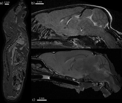
Fig. 2.
Three examples of T 2-weighted mouse images taken at 7 T. (a) A fixed whole mouse prepared by perfusion fixation with ultrasound guidance (Ref. (101)) including 10 mM Magnevist. A spin echo sequence was used with TR/TE = 650/15 ms and (100 μm)3 voxels resulting in an imaging time of 13 h. (b) A brain imaged in vivo. A fast spin echo sequence was used with cylindrical acquisition, TR/TE = 900/12 ms, with TEeff = 36 ms, echo train length 8, two averages, flip angle 40°, matrix size 400 × 240 × 240, resolution (100 μm)3 resulting in an imaging time of 2 h and 50 min (Ref. (119)). (c) A fixed brain prepared by perfusion fixation with 0.5 mM ProHance (Bracco Diagnostics, Inc.). After fixation, the skull is separated from the body. A fast spin echo sequence was used with TR/TE = 325/6 ms, with TEeff = 30 ms, echo train length 6, four averages, matrix size 780 × 432 × 432, resolution (32 μm)3 resulting in an imaging time of 11.3 h. Figure provided courtesy of Christine Laliberté.
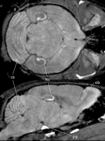
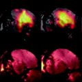
Fig. 3.
A coronal (top) and sagittal (bottom) view of an in vivo mouse brain imaged with MnCl2 injected as a contrast agent. The MnCl2 was intraperitoneally injected 24 h prior to imaging. The T 1-weighted spin echo sequence had the following scan parameters: TR/TE = 90/3.8 ms, flip angle 55°, resolution = (115 μm)3 and scan time = 2 h. With no manganese, the contrast is very flat but in the image it can be seen that the Mn2+ is taken up by the layers of the cerebellar folia (cerebellum, cb), the hippocampus (hc), the olfactory bulbs (ob) as well as in the pituitary gland (pg).
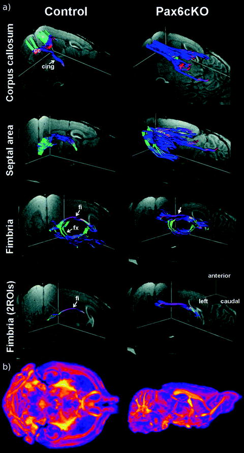
Fig. 4.
Applications of diffusion-weighted imaging in mouse brain. For color figures, please refer to the on-line version, which is available through most institutional subscriptions. (a) 3D views of major fiber pathways of a control and Pax6cKO mouse in vivo. Corpus callosum: Although controls present with a pronounced connection of the 2 hemispheres via the corpus callosum (cc) and projections into the cingulate and motor cortex, mutants reveal a strong rostrocaudal fiber orientation and a nearly complete lack of interhemispheric projections. Septal area: Mutants are characterized by a vast disorganization of fibers crossing the septal region. Fimbria: In mutants the enlarged hippocampal fimbria (fi) is shifted rostrally and exhibits a much thicker and less curved fiber structure as demonstrated by region-to-region fiber tracking (bottom). cing = cingulum; fx = fornix. Directional color code: red = left–right, blue = rostral–caudal, green = anterior–posterior. Reproduced with permission by Oxford University Press (Ref. (37)). (b) A coronal (left) and sagittal (right) view of the fractional anisotropy map in a fixed mouse brain. A 3D diffusion-weighted fast spin-echo sequence was used with an echo train length of 6 with a TR of 325 ms, first TE of 30 ms, and a TE of 6 ms for the remaining five echoes, ten averages, field of view 14 × 14 × 25 mm3 and a matrix size of 120 × 120 × 214 yielding an image with (117 μm)3 voxels. For the calculation, one b = 0 s/mm2 image (with minimal diffusion weighting) and six high b-value images (b = 1956 s/mm2) in six different directions [(1,1,0),(1,0,1),(0,1,1),(–1,1,0),(–1,0,1),(0,1,–1)] (Gx,Gy,Gz) were produced. Total imaging time was ∼16 h. Yellows indicate values closer to unity (fibers are very ordered in one direction) and deep purples indicate more isotropy. Figure provided courtesy of Dr Jacob Ellegood.
3.3.2 Imaging in the Chest and Abdomen
1.
In general, anatomy of interest distant from sites of physiological motion can be secured to prevent motion artifacts in images. For instance, we use specially cut Velcro to secure the head during brain imaging (see Fig. 1). Another simple method to minimize motion artifacts is to place the mouse in a supine position, such as for imaging of the kidneys (45) or spine.
2.
In most of the chest and abdomen, however, motion is pronounced and cannot be eliminated. Instead, imaging approaches aim to achieve a “snapshot” of the motion. This is particularly challenging as the murine heart rate is typically around 500 beats per minute and the anesthetized mouse breathes once every 1–2 s. In the past decade, several techniques have emerged to enable cardiac cine-MRI in which the ventricular size and shape can be assessed at multiple phases of the heart cycle and is discussed in much greater detail in the Chapters 20, 21, and 22.
3.
Briefly, there are typically two ways of taking images: prospectively and retrospectively. In prospective gating, the scanner is set to acquire data only during a specified phase of the heart cycle. This method is quite efficient and provides excellent cardiac images (48–50). In retrospective gating, data are continually acquired and the respiratory and ECG signals are recorded. Data are oversampled (e.g., data for more than one image are acquired) and then sorted according to cardiac phase and respiratory status retrospectively, retaining only data acquired during the quiescent respiratory period and at a specified cardiac phase (51, 52). A key benefit of the retrospective method is that multiple mice can be imaged in this fashion (53).
4.
State-of-the-art techniques to date yield cardiac images on the order of 100 × 100 μm2 with slice thicknesses at about 0.5 mm, with some groups achieving isotropic voxels (54, 55). Several disease models have been investigated, including models of myocardial infarction (56), transgenic models (57–59), and ischemia (60).
5.
Another challenging area of research is imaging the lungs in the mouse. There are typically two ways of studying the lung: using hyperpolarized inert gases to look at the airspaces (61–63) or enhancing the water signal in the lung parenchyma (64, 65). The technical knowledge and skills for set up of a hyperpolarized gas system can be significant, but the reward is images of the airspaces exclusively (see Chapters 10 and 24 for more details). Imaging the proton signal is also challenging as the microstructure of the parenchyma causes T 2* to be on the order of milliseconds. The T 1 can be shortened by adding a gadolinium-based contrast agent (66) or having the mouse breathe in oxygen (65). This way signal averaging can be applied along with cardiac gating to yield images of the parenchyma (see Fig. 5 from Watt et al.). The highest resolution images are 87 × 87 μm2 in-plane (66) and a number of disease models in the mouse have been studied including lung cancer (67–69), lung inflammation (61, 70), and cystic fibrosis (64).
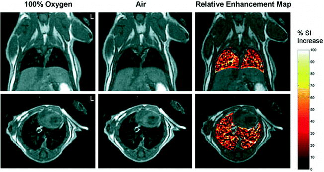
Fig. 5.
Oxygen-enhanced images of a normal mouse breathing 100% oxygen and air. For color figures, please refer to the on-line version, which is available through most institutional subscriptions. Coronal (top) and axial (bottom) images were acquired using a three-dimensional (3D) fast spin-echo (FSE) cardiac-triggered, respiratory-gated sequence with dummy scans. The relative enhancement map shows the percent increase of signal intensity in the lungs observed with 100% oxygen inhalation relative to air for images at the same slice position. To highlight signal enhancement in the lung, the intensity changes in the rest of the body have been masked. All coronal images are shown at a position dorsal from the heart and away from major vessels. Reproduced with permission from Watt et al. (Ref. (65)).
3.3.3 Contrast Agent Administration
It is beneficial in some phenotyping applications to highlight anatomy or function by administration of contrast agents that shorten the T 1 or T 2 relaxation times, producing respectively a bright (positive contrast) or dark (negative contrast) signal. There are a number of classes of contrast agents that can be used with the aim of highlighting vasculature, elucidating tumor boundaries, assessing neuronal function, or even targeting or tracking cells. These are discussed more extensively in other chapters so we discuss them only briefly here.
1.
Vascular imaging, although possible with simple pulse sequence selection (Fig. 6a), can benefit from administration of contrast agents, including chelated gadolinium (Gd) complexes and iron oxide agents. Functional information can be achieved by assessing blood inflow immediately following injection of contrast agent through a vein and then imaging dynamic changes in image contrast as the agent perfuses through the system (27, 28).
2.
3.
Assessment of functional perfusion or microvasculature parameters based on pre- and post-injection image evaluation is also being explored (73–77). Administration of vascular agents is most easily performed via intravenous tail vein injections, although alternative routes are necessary for rapid bolus injections.
4.
Neuronal function may, in some cases, be explored via administration of Mn. An intrapertioneal injection of Mn followed by a period in which mice are exposed to stimulus can modify the uptake of Mn sufficiently to show functional differences between different stimulus conditions. This has been demonstrated most clearly in the auditory system (78, 79). Focal injections of Mn or exposure of the olfactory system to Mn can also provide measurements of axonal transport and regional activity (29, 80, 81) with sufficient sensitivity to show differences in transgenic mice (82).
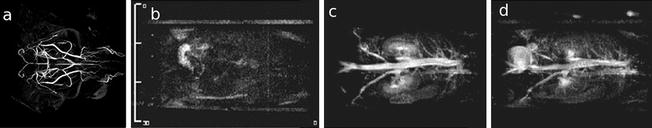
Fig. 6.
Different strategies to image the vascular system. (a) A horizontal MIP image of the adult mouse brain achieved with an inversion recovery-prepared rapid gradient echo sequence, in which the inversion time was selected to null the tissue signal and highlight blood inflow. Sequence parameters: FOV = 25.6 × 25.6 × 13.6 mm, resolution of (100 μm)3, TR = 2 s, TE = 2.9 ms, TI = 620 ms, six averages, 64 acquisitions per TR each with 12° excitation spaced 10 ms apart, total acquisition time = 1 h 49 min. Panels b–d: 3D magnetic resonance angiography (MRA) before (l) and at 4 (m) and 55 min (n) after contrast injection. With kind permission from Springer Science+Business Media: MAGMA, Contrast enhancement in atherosclerosis development in a mouse model: in vivo results at 2 Tesla, 17, 2004, 191, L Chaabane et al., part of Fig. 1 (Ref. (120)).
Significant effort continues in the development of molecular imaging, which in MRI includes applications of cell tracking, localization of targeted contrast agents, or imaging of gene expression. Successful development in this area will produce new and important in vivo phenotyping opportunities. Several genetic agents, which produce or accumulate contrast via expression of a transgene, are being explored with the hope of elucidating spatial and temporal gene expression profiles in development or disease (83–89). Alternatively, agents designed to label particular cell populations by uptake or binding to specific surface markers are also in development. Current applications in molecular imaging include detection of transgene expression in tumor-bearing mice (88, 90), integrin expression in artherosclerotic plaques (91, 92), and finding specific peptides that will attach to amyloid plaques (93) or inflammatory lesions (94). The tracking of both injected (95–99) and endogenous (31–33) cell populations after labeling with iron oxide agents shows some promise, permitting the evaluation of cellular migration behaviors in vivo during homeostasis or disease. The potential impact of genetic and cellular imaging is remarkable, motivating needed developments of these MRI methods in molecular imaging.
3.3.4 Postmortem Imaging
In vivo imaging is an extremely useful aspect of MRI. However, some studies are best served by increasing scan time to achieve microscopic resolutions in ex vivo specimens. Since the scan times can approach tens of hours, it is necessary to fix tissue to avoid degradation.
1.
To image individual organs like the brain, kidneys, and liver, the mouse is first fixed by conventional perfusion. In this procedure, mice are first anesthetized (e.g., by ketamine/xylazine) and then placed in a supine position.
2.
A midline incision through the chest is followed by catheterization of the left ventricle. A cut is also made in the right atrium and then a saline/heparin flush is followed by perfusion of a fixative solution.
3.
Including a contrast agent such as gadolinium in the perfusates also serves to reduce subsequent imaging time.
4.
The organ of interest is then excised, immersed in a proton-free, susceptibility-matching fluid and then imaged.
5.
Smaller, solenoidal RF coils can be used when imaging excised organs, which give better sensitivity.
6.
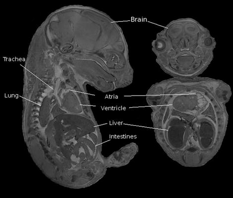
In the case of embryos, they are removed from the mother and then immersion-fixed in formalin and 4 mM MultiHance (Bracco Diagnostics Inc, Princeton, NJ) for 3 days and then transferred to 1% agarose. Figure 7 shows an example of a 15.5-dpc (days post coitum) embryo imaged in this fashion.
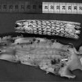
Fig. 7.
Sagittal (left) and coronal views of a 15.5-dpc mouse embryo. A gradient echo scan was used with the following scan parameters: TR/TE =50/5.06 ms, flip angle 60°, FOV = 2.5 × 1.4 × 14 cm, resolution is (32 μm)3, six averages for a total scan time of about 14 h.
To image the whole mouse adult body, it is desirable to avoid damage to the thoracic cavity and two techniques have emerged to perfusion fix the mouse without breaching the chest cavity.
1.
One method involves cannulating the right jugular vein and the left carotid artery and passing the perfusates through these points (100).
2.
The other uses an ultrasound biomicroscope to guide the catheter into the left ventricle, allowing the mouse to be fixed in much the same fashion as the open-heart perfusion fixation, with the exception that the perfusates are drained through cuts in the femoral and jugular veins (101). Figure 2a shows an MR image of a mouse fixed in such a fashion.
3.4 Anatomical Image Analysis
Figure 8 shows several examples of different phenotyping analyses for MRI that will be discussed below, as applied to neuroanatomical mutants (reproduced from Nieman et al. (21)). Briefly, the panels (a) and (b) show significant local volume changes; panels (c) and (d) show two illustrations in which a phenotype is immediately recognizable by eye; panels (e) and (f) are more subtle mutant phenotypes which require detailed statistical analyses for identification.
Fig. 8.
Neuroimaging findings in mouse mutants. For color figures, please refer to the on-line version, which is available through most institutional subscriptions. In (a), an average control mouse image is shown with two Jacobian overlays indicating local volume changes in the heterozygous and homozygous wobbly mutants. Values greater or less than 1 in the Jacobian field represent growth or shrinkage, respectively. Jacobian overlays in panel (a) are shown in regions where p < 0.05 with white contour lines indicating p = 0.002 (a false discovery rate of 5% in the homozygous mutant). The average homozygous wobbly mutant image is also shown for reference and exhibits a small cerebellum. In (b), data from the EphB2 knockout study indicates an abnormality at the anterior commissure (the posterior portion is absent). Jacobian data in the middle image indicate regions where p < 0.003 (5% false discovery rate). Panel (c) shows two sample micro-CT datasets as maximum intensity projections. The cerebral ischemia mutant shows a striking defect in vascular perfusion as compared to the control. Panels (d) and (e) provide two examples of hydrocephalus. Three different individual images from the sonic hedgehog pathway mutation are shown (d) with massive expansion of the ventricles (shown as hypo-intense regions). In panel (e), control and mutant averages from the bobbing head study show more subtle ventricle expansion (shown as hyper-intense regions). In this case, statistical comparison of the mutant Jacobian values to a set of 20 control mice (four wildtype littermates supplemented with non-littermate wildtypes) shows expanded ventricles (regions indicate a 5% false discovery rate) and increased variability at the lateral ventricles (Jacobian variance ratio is shown in regions where p < 0.05). In the final panel (f), regions of abnormality representative of the disrupted-in-schizophrenia-1 mutants (Disc1) are shown as Jacobian data overlaid on an average image (regions indicate p < 0.05 by a Mann–Whitney U test). All white scale bars indicate 2 mm. Color scales are indicated in panels (a), (b), (e), and (f) for the respective overlays. Data were acquired with in vivo magnetic resonance imaging (MRI) (panels a, d, and e), ex vivo specimen computed tomography (c), ex vivo specimen MRI (d), and in situ specimen MRI (f). All MRI images are single slices from three-dimensional isotropic datasets. Reproduced with permission from Nieman et al. (Ref. (21)).
3.4.1 Basic Quantitative Measures
After acquiring image data for a study, the main challenge is quantitative data analysis. A human observer can make qualitative observations (e.g., “the left ventricular wall is thicker than the wildtype” or “the tumor looks bigger in one mouse compared to another”) but the real power of MRI is that quantitative measures can be obtained from the images.
1.
Using freely available image processing packages, the previous examples can easily be quantified by measuring the wall thicknesses and segmenting tumor volumes. Most visualization packages have a manual segmentation feature and many have some form of semi-automatic segmentation.
2.
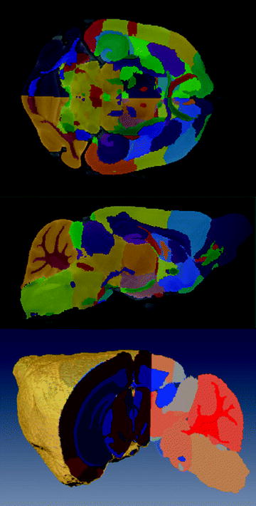
If the subject numbers are few, manual segmentation is rapid, reliable, and widely utilized (7, 46, 51). An advantage is that it does not require any knowledge or development of more elaborate image processing methods. Figure 9 shows an example of manual labeling of 62 substructures in the mouse brain (102).
3.
Typically small, simple structures (e.g., the anterior commissure in the brain) can be segmented in tens of minutes as they only occupy a few slices within a dataset.
4.
Segmenting more expansive structures like the corpus callosum or hippocampus can take more than an hour. If many mice are part of the study, manual segmentation on all subjects is prohibitive; hence using computer-aided image processing tools is prudent.
Fig. 9.
Three views from a manual segmentation of 62 sub-structures from an average of 40 mouse brains (Ref. (102)). For color figures, please refer to the on-line version, which is available through most institutional subscriptions. The brains were from 20 male and 20 female 12-week-old C57Bl/6 J mice. Three brains were imaged in parallel with a fast spin echo sequence (TR/TE = 325/32 ms, four averages, (32 μm)3 resolution for a total scan time of 11.3 h. The top and middle panels show coronal and sagittal slices (respectively) of the atlas overlaid on top of the average. The bottom panel is a 3D volume rendering with a cutout showing the segmentation (a different colormap was used than the previous two panels).
3.4.2 Registration
It is frequently impractical to perform manual segmentation of volumes for image analysis, and, in these cases, it is common to make use of registration algorithms to elucidate any disparities. The registration process produces transformed images that are aligned with one another such that common structures are placed on top of one another, in “register.” The image transformations required to achieve such alignment encode phenotypic differences. The phenotypes can be extracted from registration-based analyses in several ways, based on structural volumes as described above or on more sophisticated voxel-by-voxel measurements of shape or size differences.
1.
 Spin Echo BOLD fMRI on Songbirds
 Interventional MRI in the Cardiovascular System
 Analysis of Freshly Fixed and Museum Invertebrate Specimens Using High-Resolution, High-Throughput MRI
 MRI Using Intermolecular Multiple-Quantum Coherences
 MRI of CEST-Based Reporter Gene
 Hyperpolarized Molecules in Solution


A number of registration packages are listed in Section 2.5, item 3. In general, the registration process begins by first globally aligning images through affine registration, which includes global translations, rotations, scales, and shears. These modifications are considered linear operations and are applied to the entire image (see Note 8).
Related posts:
Spin Echo BOLD fMRI on Songbirds
Interventional MRI in the Cardiovascular System
Analysis of Freshly Fixed and Museum Invertebrate Specimens Using High-Resolution, High-Throughput MRI
Hyperpolarized Molecules in Solution
Stay updated, free articles. Join our Telegram channel
Full access? Get Clinical Tree
