Fig. 1.
Schematic representation of the vertebral segments and sagittal, coronal, and axial MR images of the spinal cord at the cervical, thoracic, and lumbar levels. The arrows (sagittal and coronal views) and squares (axial view) indicate the spinal cord.
The spinal cord is composed of gray matter (GM) and white matter (WM). The gray matter is made up of neuronal cell bodies, dendrites, axons, and glial cells and it can be divided into dorsal, intermediate, and ventral horns, and central gray matter around the central canal (Fig. 2c). Gray matter is bordered by white matter at its circumference (Fig. 2d), except at locations where the dorsal horns touch the margin of the spinal cord. The white matter consists mostly of longitudinally running axons and glial cells and it is conventionally divided into the dorsal, dorsolateral, lateral, ventral, and ventrolateral funiculi. The spinal cord is enclosed by a tube of cerebrospinal fluid (CSF) and protected by three membranes called the spinal meninges (Fig. 2b).
Fig. 2.
Axial MR image of the spinal cord and schematic representation of the structures.
In rodents, the overall diameter of the spinal cord ranges from 2 to 3 mm. The small size of the spine and its surrounding bony structure render mouse or rat SC MRI comparatively challenging.
For further details on the structures and nomenclature, the reader can refer to available atlases of rat and mouse spinal cord (2).
2.2 MR Systems and rf Coils
1.
High-field micro-imaging systems are adapted to SC investigation since they offer both high MR signal compared to clinical scanner fields (1.5 T or 3 T) and strong gradient performance. Such dedicated small animal systems are therefore of great help for achieving adequate resolution and signal-to-noise ratio (SNR). Some studies carried out on clinical scanners have been reported (3–5) and the readers can refer to these earlier studies to obtain more information on protocols using those MR systems. However, most of the rodent studies have been performed with dedicated small animal MR systems at 4.7 T (6–14), 7 T (15–20), and 9.4 T (21–30). Although, very high field systems are not yet widely present in labs, studies at 11.75 T (31–36) and 17.6 T (37–39) have been reported successful.
2.
Since MR microscopy requires strong field gradients, actively shielded gradient systems with integrated shim coils and high performances, including high gradient strength, short gradient slew rates, good gradient duty cycle, optimal gradient linearity, and high gradient shielding quality, are recommended, especially when using rapid imaging techniques such as echo planar imaging (EPI) sequences. The combination of diffusion gradients with EPI readouts requires a reliable gradient pre-emphasis unit.
3.
Beyond high-field magnets, well-adapted radio frequency (rf) coils should be considered for an optimized MR SC investigation. Although many studies reported in the literature were carried out using conventional small animal transmit–receive volume coils (17, 32), transmit–receive surface coils (38), and separate transmit and receive coils (geometric or active decoupling) (8, 27), much effort has been put into investigation of highly specialized implantable coils (21, 40), phased arrays (18) or cryogenic probes (41). All coil systems have proven to be applicable in SC studies, but their advantages and disadvantages may lead an investigator to choose one system over the others. Implantable coils provide excellent SNR, but the procedure is invasive and surgery may be difficult in the deeper cervical region. Surface coils offer limited spatial coverage but generally good SNR. Volume coils are suitable for large screening purposes offering increased spatial coverage and good field homogeneity but lower SNR as compared to surface coils. Phased arrays offer both high SNR and spatial coverage and they provide parallel imaging capabilities, which can be helpful for a better motion robustness of various imaging techniques.
2.3 Animal Handling
1.
Anesthesia: In most of the studies, animals are kept anesthetized by spontaneous respiration of a mixture of air and isoflurane through a nose cone. Flow rate (250–300 mL/min) and isoflurane concentration (1.5–2%) have to be optimized to obtain a regular breathing. A mixture of intraperitoneal ketamine (80 mg/kg) and xylazine (10 mg/kg) can also be used.
2.
Temperature regulation: In small-bore systems, the physiological temperature can be maintained by heating the gradient cooling system to appropriate temperatures. In larger bore systems, a warming pad must be used.
3.
Animal positioning: Animals are positioned on an animal bed usually in prone position for mice and supine for rats. A MRI-compatible device designed to immobilize the spinal column and suspend the lower body of the animal may eventually be used to isolate respiratory motion from the cord (8). In vertical MR systems, the animals are positioned head up and maintained using a teeth holder and by taping the neck and pelvis to the cradle. No other restraining device is necessary (32).
4.
Physiologic monitoring: In order to minimize motion artifacts in the MR images, the respiratory signal is taken from a pressure sensor connected to an air-filled balloon placed under the abdomen of the animal (Rapid Biomedical (Rimpar, Germany) or SA instruments (Stony Brook, NY, USA)) and acquisitions are synchronized with breath motion.
2.4 Post-processing Software
1.
For relaxation time map calculation (T 1, T 2, or  ), home-built programs capable of performing pixel-by-pixel fitting of the function S(t) = f(T 1, T 2, or
  ) to the serial images data acquired with the MR system, are needed. Programming toolkits such IDL (Interactive Data Language, ITT Visual Solutions, Boulder, CO, USA) or MATLAB (Mathworks, Natick, MA, USA) are well adapted. These toolkits also provide helpful libraries for analyzing the metrics in different regions of interest.
), home-built programs capable of performing pixel-by-pixel fitting of the function S(t) = f(T 1, T 2, or ) to the serial images data acquired with the MR system, are needed. Programming toolkits such IDL (Interactive Data Language, ITT Visual Solutions, Boulder, CO, USA) or MATLAB (Mathworks, Natick, MA, USA) are well adapted. These toolkits also provide helpful libraries for analyzing the metrics in different regions of interest.2.
The DTI metrics can usually be calculated directly on the MR system (e.g., the “DTI_proc_tensor” macro on Bruker ParaVision 3.02) or by using dedicated software such as FSL (42) (http://www.fmrib.ox.ac.uk/fsl/).
3.
The MRS data may be analyzed using the magnetic resonance user interface software package (MRUI, http://sermn02.uab.cat/mrui/) or the LCModel software (http://s-provencher.com/pages/lcmodel.shtml).
3 Methods
This paragraph provides an overview of the principal MR applications useful to study spinal cord in rodent models. They mainly include T 1 and T 2-w imaging for the morphology, diffusion tensor imaging for the tissue structure, and perfusion imaging for the hemodynamics.
These MRI techniques, which can be performed in most of the MR systems, allow obtaining significant in vivo information on the pathophysiology and recovery mechanisms involved in spinal cord diseases. Advances in MR technology, such as more powerful gradient systems, refined rf coil design, and new sequence designs, will provide increased sensitivity and faster acquisition. Therefore, in the near future, MRI studies, in combination with other imaging modalities and histology, are expected to play an increasing role in the delineation of pathophysiologic mechanisms, the characterization of novel therapeutic strategies, and the longitudinal assessment of recovery mechanisms.
3.1 Preparation Scans
1.
Scout images are acquired to check the animal position inside the coil and to provide a localization reference. The SC segments of interest have to be positioned in the magnet center.
2.
Spectrometer adjustments such as tuning and matching of the rf coil, base frequency, reference rf gain, and shimming are performed at a level of automation depending on the MR scanner.
3.
A preliminary sagittal gradient echo image of high spatial resolution may be acquired as further localization reference. A strict sagittal image with clear delineation of the disks and segments can be obtained when the sagittal slice crosses the spinal canal and the spinous process.
3.2 Anatomic MRI
3.2.1 Spin Echo Sequences – T1 and T2 Measurements
T 1 – and T 2 -weighted imaging: Conventional spin echo (c-SE) or EPI-based spin echo sequences (SE-EPI, see Notes 1–3) can be used with appropriate repetition time (TR) and echo time (TE) to obtain different useful image contrasts (see Table 1). T 1– and T 2-weighted images allow size and volumetric evaluation and provide complementary information on the pathology. T 1-weighted images optimally highlight normal soft-tissue anatomy and fat, whereas T 2-weighted images optimally highlight the presence of fluid and pathology (e.g., tumors, inflammation, trauma, and edema). Examples of T 1 and T 2-weighted images are given in Fig. 3.
T 1 calculation: T 1 values can be calculated by using a saturation or an inversion recovery SE technique, with increasing TR or inversion time (TI), respectively. Examples of protocol are given in Table 2.
T 2 calculation: T 2 values can be measured by using a multi-spin echo (MSE) sequence, but one major problem of this approach is potential contamination of the spin echo train by stimulated echoes if the 180° refocusing pulse is imperfect. To limit this contamination, acquisitions are often performed separately for each TE (TE-step method). Examples of T 2 protocols are given in Table 2.
T 1 and T 2 values of gray and white matter at different magnetic fields are summarized in Table 3. Examples of T 1 and T 2 maps are given in Fig. 3b and d.
Proton density calculation: Although not frequently used, proton density measurements can also be performed. They are in some cases necessary for calibration purposes when quantitative MR parameter information is required. The protocol and typical values are indicated in Tables 2 and 3, respectively.
Fig. 3.
Healthy mouse T 1 and T 2-weighted imaging at 11.75 T, at the cervical level. From left to right: (a) T 1-weighted images for different TI and (b) resulting T 1 map. (c) T 2-weighted images for different TE and (d) resulting T 2 map. T 1 values are in the order of 1870 and 1820 ms in the GM and WM, respectively. T 2 values are around 28 ms in GM and 40 ms in WM.
Table 3
T 1, T 2, and PD values measured at different magnetic fields
Normal values (healthy rodents) | ||||||
|---|---|---|---|---|---|---|
T 1 (ms) | T 2 (ms) | PD (%) | ||||
Magnetic field | WM | GM | WM | GM | WM | GM |
2 T (40), * | 1089 | 1021 | 79 | 64 | 40 | 60 |
7 T (17), * | 57 | 43 | ||||
9.4 T (24), + | 1690 | 1730 | 38 | 33 | 44 | 56 |
11.75 T (32), + | 1820 | 1870 | 40 | 28 | ||
Table 1
Relation between TR, TE, and image contrast for a spin echo sequence
MR parameters | Short TR | Long TR |
|---|---|---|
Short TE | T 1 | PD |
Long TE | T 1, T 2 | T 2 |
Table 2
Protocols for T 1, T 2, and PD measurements in the axial plane. See Note 3 for additional comments on the EPI acquisitions
Spin echo sequence – T 1 and T 2 relaxometry | ||||
|---|---|---|---|---|
Animal model | Rat | Mouse | ||
References | (40) | (17) | (32) | (24) |
Readout/sequence | SE-EPI | c-SE | SE-EPI | c-SE |
rf Coil | Implanted coil | Birdcage coil | Birdcage coil | Inductively-coupled surface coil |
Magnetic field (T) | 2 | 7 | 11.75 | 9.4 |
FOV (mm²) Matrix Slice thickness (mm) | 25 × 25 128 × 128 2 | 15 × 30 64 × 128 3 | 17 × 17 128 × 128 0.75 | 12 × 8 64 × 64 2 |
T 1 measurements | Saturation recovery | – | Inversion recovery | Saturation recovery |
TR (s) | 0.3a, 0.5a, 0.7a, 1.0, 2.0, 3.0, 5.0 | 10 | 0.25, 0.50, 0.75, 2.0, 3.5, 6.0 | |
TI (s) | 0.13, 0.53, 0.9, 1.4, 1.7, 4, 9.0 | |||
TE (ms) | 25 | 10.7 | 12 | |
# of averages | 2 or 4a | 9 | 2 | |
T 2 measurements | TE-step | TE-step | TE-step | TE-step |
TR (s) | 1.0 | 2.5 | 10.0 | 4.0 |
TE (ms) | 25, 30, 35, 40, 60a, 80a | 10, 20, 40, 60, 80, 100, 120 | 20, 30, 50, 60, 70 | 12, 24, 36, 48 |
# of averages | 2 or 4a | 2 | 5 | 2 |
PD measurements | ||||
TR (s)/TE (ms) | 5/25 | 6/12 | ||
3.2.2 Gradient Echo Sequences –  Measurements
 -weighted imaging: Gradient echo sequences may be advantageous when using surface coils for transmission because they are less sensitive to rf field inhomogeneities.
  -weighted images may also help in lesion detection. An inflammatory lesion will appear as a hyper-intense area in the normal-appearing white matter and hemorrhage will present as hypo-intense area on the images. Examples of gradient echo images are given in Fig. 4a (healthy SC) and 4b (contused SC).
 calculation:
  relaxation measurement may, for example, be exploited when iron-based contrast agents are employed, i.e., when labeling cells with small iron oxide particles.


Fig. 4.
(a) Healthy rat gradient echo imaging at 17.6 T at the lumbar level. (b) Gradient echo image of contused rat SC at mid-thoracic level. The hypo-intense structure, which is due to hemorrhage, represents the lesion center, with disruption of the normal GM/WM. (c) Healthy rat  map of the spinal cord. Values range from 5 to 20 ms. A ventral to dorsal
  -gradient resulting from distortion of the magnetic field by the nearby bony structures is visible. Modified from Ref. (38), copyright [2004], with permission from ESMRMB and acknowledgment to V. Behr (Wuerzburg, Germany).
map of the spinal cord. Values range from 5 to 20 ms. A ventral to dorsal -gradient resulting from distortion of the magnetic field by the nearby bony structures is visible. Modified from Ref. (38), copyright [2004], with permission from ESMRMB and acknowledgment to V. Behr (Wuerzburg, Germany).Table 4
Protocol for  measurement and gradient echo imaging
measurement and gradient echo imagingGradient echo sequence –  relaxometry relaxometry | |
|---|---|
Animal model | Rat |
Ref. | (38) |
rf coil Magnetic field (T) | Transmit–receive surface coil 17.6 |
FOV (mm²) Matrix Slice thickness (mm) | 24 × 24 192 × 192 0.5 |
# of echoes | 8 |
TR/TE/inter-echo spacing (ms) | 200 /2.75 /3.9 |
# of averages | 32 |
3.3 Diffusion MRI
In addition to the standard contrasts (T 1, T 2, and PD), diffusion MRI provides excellent differentiation between gray and white matter due to the differences in mobility that the water molecules experience during their random walk in the microscopic tissue organization (43, 44). Diffusion-weighted imaging (DWI) and diffusion tensor imaging (DTI) (43) thus offer helpful information about tissue micro-architecture. The changes in the metrics that can be derived from such experiments (fractional anisotropy and directional diffusivities, see Note 4) usually correlate with pathophysiologic changes and the histopathology. DTI metrics may especially be seen as a complement to routine imaging, since variations may show tissue alteration or disruption in regions that appear normal on the conventional MRI (16, 45), suggesting the potential of the technique in detecting subtle pathology.
DWI : The diffusion techniques in rodent studies are usually based on c-SE, however SE-EPI techniques have also been proven to work for both rat and mice studies (18, 33, 36, 46) (see Note 1). Diffusion contrast is obtained by adding diffusion gradients during the preparatory phase of an imaging sequence. Many of the reported diffusion measures were determined from the diffusion-weighted images acquired with gradients applied parallel and perpendicular to the axis of the magnet (13, 15, 17, 26, 30, 47) rather than on the complete determination of the diffusion tensor. Resulting contrasts are illustrated in Fig. 5.
DTI : DTI is widely used to explore the brain and its application to SC investigation has considerably increased during the last 5 years. DTI is particularly useful for assessing alterations in WM tracts occurring in multiple or amyotrophic lateral sclerosis (7, 8, 31, 48, 49), as well as those occurring after SCI or infarction (7, 9, 16, 26, 50–52). DTI could also help to characterize glial processes in the GM adjacent to the site of injury (51). In general, it has been demonstrated that decreased axial diffusivity is associated with axonal injury and dysfunction and increased radial diffusivity with myelin injury (11, 53).
To acquire DTI data, use parameters as given for different protocols in Table 5. The DTI metrics that can be derived from such measurements are presented in Table 6.
DTI and MS: In multiple sclerosis models, decrease in axial diffusivity (λ //) has been demonstrated to be associated with altered axon and increase in radial diffusivity (λ ⊥) with loss of integrity of myelin (8).
DTI and SCI: In SCI models, DTI metrics are also essential for quantifying the direct mechanical damage of the cord (7, 9, 13, 16, 19, 26, 39, 50, 53–56), evaluating the secondary injury, predicting functional outcomes (57), and to test regenerative strategies (1, 28, 29, 58). At the lesion site, increased radial diffusivity in both GM and WM reflects the disruption of cell membranes and myelin sheaths. Increase in the axial diffusivity for GM shows disintegration with hemorrhages and disappearance of normally discernable cellular elements, whereas decrease in WM is associated with mechanical disruption of neural tissues. DTI also allows quantification of the asymmetric rostral and caudal variations associated with the regional extent of the injury, swelling processes, cyst formation, and secondary excitotoxic processes (59). An illustration of DTI applied to SCI model is given in Fig. 6.
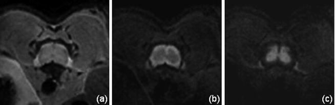
Fig. 5.
Mouse spinal cord transverse images at 11.75 T, without diffusion gradient (a) and with gradient (b = 800 s/mm²) applied perpendicular (b) and parallel (c) to the spinal cord axis. The observed contrast between WM and GM (b, c) is in agreement with the preferential alignment of the WM fibers along the SC axis.
Fig. 6.
(Top) Pre and post-injury relative anisotropy (RA) maps at the injury site (T12), demonstrating the temporal evolution of acute spinal cord injury. (Bottom) Axial (//) and radial (┴) mean diffusivity variations, calculated in ROI outlined in white, for the pre-injury control and 1, 3, 7, and 14 days post-injury (DPI). The observed variations at the epicenter, the existing rostral–caudal asymmetry (data not shown), and the transient changes, suggest that DTI provides a sensitive tool for monitoring the dynamic pathophysiologic processes that occurs after SCI. Modified from Ref. (9), copyright [2007], with permission from Wiley and acknowldgements to S-K Song (St-Louis, USA).
Table 5
Protocols for DTI acquisitions in the axial plane. Additional comments are given in Notes 3 (EPI sequence), 5 (bulk motion), 6 (SNR consideration), and 7 (diffusion-encoding directions)
Diffusion tensor imaging | ||||
|---|---|---|---|---|
Animal species | Rat | Mouse | ||
References | (46) | (27) | (33) | (8) |
Readout/sequence | EPI / SE (8-shots) | c-SE | EPI / SE (4-shots) echo position 18% | c-SE |
rf coil | Implanted coil inductively coupled to an external coil | Volume transmit coil and surface receive coil | Volume coil | Surface coil inductively coupled to an Helmholtz coil |
Magnetic field (T) | 2 | 9.4 | 11.75 | 9.4 |
FOV (mm²) Matrix Slice thickness (mm) | 25 × 25 12 8 × 80 2 | 38.4 × 38.4 128 × 128 2 | 12.8 × 12.8 + 2 OVS 128 × 128 0.75 | 10 × 10 128 × 128 0.75 |
TR (ms) | 2000 | 500 | 3500 | 1200 |
TE (ms) | 60 | 31 | 15.25 | 38 |
# of directions | 6 (1,0,0),(0,1,0),(0,0,1),(√2/2,√2/2,0),(√2/2,0,√2/2),(0,√2/2,√2/2) | 6 (±0.33,0.67,0.67),(0.67,±0.33,0.67),(0.67,0.67,±0.33) | 6 (1,±1,0),(1,0,±1),(0,1,±1) | 6 (±1,1,0),(1,0,±1),(0,±1,1) |
b-Values (s/mm²) | {0, 750–1000} | {0, 1000} | {0, 700} | {0, 785} |
δ/Δ (ms) | 13/26 | 3/15 | 2.3/6.8 | 7/20 |
# of averages | 4 | 1 | 18 | 8 |
Synchronization | Respiration | Respiration | Respiration | Respiration |
Table 6
Examples of DTI metrics derived from DTI measurements on healthy rodents. Additional comments are given in Notes 8 (ROI location), 9 (in vivo vs. ex vivo), and 10 (fast and slow components)
Normal values | FA | λ // (10–3 mm²/s) | λ ⊥ (10–3 mm²/s) | |||||
|---|---|---|---|---|---|---|---|---|
Species | Level | WM | GM | WM | GM | WM | GM | |
Rat | Cervical | C3:C7 (18) | 0.82 ±0.05 | 0.36 ±0.04 | 2.15 ±0.26 | 1.54 ±0.20 | 0.33 ±0.05 | 0.83 ±0.06 |
C3 (27) | 0.70 ±0.01 | 0.59 ±0.01 | 0.85 ±0.01 | 0.72 ±0.01 | 0.23 ±0.01 | 0.26 ±0.01 | ||
Thoracic | T7:T12 (18) | 0.83 ±0.05 | 0.38 ±0.04 | 1.94 ±0.12 | 1.49 ±0.11 | 0.29 ±0.07 | 0.77 ±0.12 | |
T8 (27) | 0.62 ±0.01 | 0.57 ±0.01 | 0.72 ±0.01 | 0.71 ±0.01 | 0.25 ±0.01 | 0.28 ±0.01 | ||
Caudal | Equine (27) | 0.56 ±0.01 | 0.97 ±0.02 | 0.38 ±0.01 | ||||
Mouse | Cervical | C1:C6 (36) | 0.83 ±0.02 | 0.27 ±0.02 | 2.03 ±0.12 | 1.03 ±0.04 | 0.31 ±0.01 | 0.69 ±0.02 |
T6–T10 (28) | 0.80 ±0.08 | 0.36 ±0.11 | 1.37 ±0.12 | 0.72 ±0.12 | 0.26 ±0.11 | 0.42 ±0.04 | ||
Thoracic/lumbar | T8–T12 (24) | 0.76 ±0.09 | 0.61 ±0.07 | 1.95 ±0.13 | 1.25 ±0.11 | 0.46 | 0.48 | |
T10–L2 (33) | 0.71 ±0.03 | 0.30 ±0.02 | 1.82 ±0.08 | 1.08 ±0.07 | 0.48 ±0.05 | 0.69
Related posts:Stay updated, free articles. Join our Telegram channel
Full access? Get Clinical Tree
 Get Clinical Tree app for offline access

| ||