Fig. 6.1
(a) MRI of a phantom containing main brain metabolites dissolved in a water-based, pH-buffered stock solution. (b) Spectrum acquired from the VOI prescribed in a using volume-selective spectroscopy sequence with PRESS excitation (TR: 2000 ms, TE: 35 ms)
The information obtained during MRS experiments, usually acquired as a series of FIDs, spin echoes or stimulated echoes in the time domain, is displayed graphically as a spectrum in the frequency domain with individual peaks representing the various chemical compounds. The diagnostic ability of MRS can be increased by improving the spectral quality through changes in hardware and software and/or by improving the analytical approach aiming for objective absolute concentration measurements.
MRS should be performed as an adjunct to MRI gain additional information for a reliable clinical diagnosis: while conventional MRI provides anatomical images of the brain, MRS provides functional information related to its underlying dynamic physiology.
6.1 Spectroscopy Basics
MRS has been demonstrated in vivo for different nuclei, including 1H, 31P, 13C, 15N, 19F and 23Na. While most of these nuclei are very difficult to detect, 1H and 31P are available in the human brain in significant concentrations and have the appropriate physical configuration to be detected by MRS. Besides the technical prerequisites, 1H and 31P are prominent candidates for clinical studies also from a biochemical viewpoint, as they allow in vivo investigation of some of the processes involved in brain metabolism. For instance, 31P-MRS has been the first to be applied to medicine in vivo and can be used to evaluate brain energy metabolism by directly and non-invasively measuring ATP, PCr or Pi concentrations. While 31P-MRS was the first spectroscopic technique to be applied in vivo, the main nucleus studied today in neurospectroscopy is 1H, which provides information on markers of neurons, myelin, energy metabolism and other metabolically active compounds. Besides its important clinical role, 1H spectroscopy is also less technically demanding as it uses hardware employed for standard MRI and provides a higher signal/noise ratio (SNR) [1, 3].
6.1.1 Proton MRS in Neuroradiology
Proton magnetic resonance spectroscopy of the brain reveals specific biochemical information about cerebral metabolites, which may support clinical diagnosis and enhance the understanding of neurological disorders. Analysis of the resonance signals of low-molecular-weight brain metabolites (concentrations in mmol) provides information on metabolite concentrations and makes it possible to correlate their modifications with various pathological conditions. The high diagnostic specificity of MRS enables the biochemical changes that accompany various diseases to be detected, as well as disease characterization, sometimes diagnosis and monitoring. At 1.5 T the main metabolites detected vary according to the acquisition parameters (TR, TE) and type of pulse sequence adopted (STEAM, PRESS). 1.5 T brain MRS currently has a number of clinical applications, including the characterization of cerebral tumours and the monitoring of their treatment (e.g. radiation necrosis versus recurrence tumour), epilepsy, infection, stroke, multiple sclerosis (MS), trauma and neurodegenerative processes, such as Alzheimer’s and Parkinson’s diseases [2–5], and allows to diagnose several hereditary and acquired brain metabolic disorders such as Canavan’s disease [6], brain creatine deficiency syndromes [7, 8], adrenoleukodystrophy [9] and hepatic encephalopathy [10].
However, despite the demonstrated ability of MRS to detect neurochemical changes and to be technically feasible to study the brain in vivo, there are no standardized techniques for acquiring and interpreting MRS spectra, and little high-quality direct evidence of its influence on diagnosis and therapeutic decision-making is available. Its specificity, diagnostic and prognostic value needs to be improved, and especially its sensitivity to disease markers, all of which can be achieved at higher magnetic field.
In the recent past, high magnetic field MR systems, particularly 3 T instruments, have proliferated with FDA “non-significant risk” clearance [11] and have replaced 1.5 T in many clinical and research applications now performed with these magnets [12]. 1.5 T fields have long been seen as the standard, but the development of 3 T and higher-field technology suggests that the concept of “high field” may be a moving target. Indeed, NMR spectrographs operating at magnetic fields of 14–21 T are routinely used for in vitro structural studies of complex molecules. The development of in vivo high-field MRS has however been delayed by safety considerations, hardware limitations (such as the availability of wide-bore magnets), high-performance gradients and methods to correct magnetic field inhomogeneity [12, 19]. MRS like other advanced MR techniques to study the brain (e.g. angiography, diffusion, perfusion and functional imaging) should considerably benefit from the greater SNR and contrast/noise ratio and the increased spatial and temporal resolution provided by high-field systems [11–18].
Several studies comparing brain 1H-MRS at different field strengths in the same subjects using the same experimental parameters have demonstrated the usefulness of high-field 1H-MRS [19–25]. Its advantages rest on greater SNR and spectral resolution, which afford greater spatial and temporal resolution and enable the acquisition of high-quality, easily quantifiable spectra in acceptable acquisition times. In addition to improved measurement precision of common metabolites, such as N-acetylaspartate (NAA), choline (Cho), creatine/phosphocreatine (Cr/PCr), myo-inositol (mI) and when present lactic acid (Lac) and lipids (Lip), high-field systems allow the high-resolution measurement of other metabolites, such as glutamate (Glu), glutamine (Gln), glutathione (GSH), γ-aminobutyric acid (GABA), scyllo-inositol (ScyI), aspartate (Asp), taurine (Tau), N-acetylaspartylglutamate (NAAG) and glucose (Glc), thus extending the range of metabolic information. However, these advantages may be hampered by intrinsic field-dependent technical difficulties, such as increased T2 signal decay, chemical shift dispersion errors, J-modulation anomalies, increased magnetic susceptibility, eddy current artefacts, limitations in the design of homogeneous and sensitive radiofrequency coils, magnetic field instabilities and safety issues. Several studies have demonstrated that these limitations can be overcome, suggesting that optimization of high-field 1H-MRS can lead to its broader application in clinical research and diagnosis.
Table 6.1 summarizes several metabolites involved in brain biochemistry detectable with 1H-MRS. Besides the most prominent resonances of NAA, choline and creatine, a variety of other resonances might or might not be present in a spectrum depending on its type and quality as well as disease. This list is not complete, in that several metabolites are only observed in the rare cases when their concentrations are several times higher than normal, while metabolites such as alcohol and propylene glycol are not present in normal brain metabolism but may be found in certain patients. For a full list of detectable metabolites, the reader required to interpret spectra with unusual resonances is referred to the literature.
Table 6.1
Some of the primary resonances found in 1Hbrain spectroscopy and corresponding chemical shifts (in ppm)
Brain metabolites detected on 1H MRS | ||
|---|---|---|
Compound | Abbreviation | Frequency (ppm) |
Alanine | Ala | 1.48, 3.78 |
Aspartate | Asp | 3.9, 2.69, 2.82 |
Choline | Cho | 3.22 (4.05, 3.54) |
Creatine/phosphocreatine | Cr/PCr | 3.03, 3.95 |
γ-Aminobutyric acid | GABA | 2.31, 1.91, 3.01 |
Glucose | Glc | 3.43, 3.84 (…) |
Glutamate | Glu | 3.77, 2.06, 2.38 |
Glutamine | Gln | 3.71, 2.15, 2.46 |
Glycine | Gly | 3.56 |
Lactate | Lac | 1.33 |
myo-Inositol | mI | 3.56, 4.06 |
N-Acetylaspartate | NAA | 2.02 |
scyllo-Inositol | ScyI | 3.35 |
Taurine | Tau | 3.44, 3.38, 3.32, 3.27 |
6.1.2 MR Spectroscopy: Quality and Resolution
While the 1H protons bound to the H2O molecule provide basically the whole signal used for MR imaging, the high water signal is one of the most disrupting elements in MRS, since the molecules of interest are found at much lower concentrations, yielding signal amplitudes more than 1000-fold smaller than the signal of water (Fig. 6.2). Thus the quality of a spectrum, which is usually measured as SNR, and its resolution, which includes the spectral, spatial and temporal dimensions, play a major role in the applicability and acceptance of MR spectroscopy.

Fig. 6.2
a Full water signal of a phantom spectrum containing the main brain metabolites compared to the metabolite signal b several orders of magnitude smaller than the water signal
6.1.2.1 Signal/Noise Ratio
The SNR is based on several variables, the most important of which are of course signal intensity (where Cr is often used as the reference) and the underlying noise of a spectroscopy experiment. The dependencies of signal intensity and noise can be divided into two categories:
- 1.
Dependencies which cannot be affected by the user and which are given by fixed natural constants. The corresponding SNR shall be called SNRint.
- 2.
Dependencies that can be altered by modifying the acquisition parameters. The corresponding SNR shall be called SNRExp.
The most important factors for SNRint in an 1H-MRS experiment are to be aware of the number of protons contributing to the total signal N, the field strength of the static magnetic field B 0 and the relaxation properties of a specific metabolite. With a direct, linear proportionality of SNRint to N and B 0, these parameters define the intrinsic SNR available for the spectroscopy experiment, which means that an increase in B 0 from 1.5 to 3.0 T will theoretically boost the SNR by a factor of two. This achievable SNR will always be degraded by the natural phenomena of relaxation, expressed as an exponential signal decay after full excitation with the relaxation constants T2 and exponential return of the spin system into thermal equilibrium with the time constant T1.
For a given sample in a specific MR scanner, the value of SNRint is fixed, and its limitations cannot be overcome. Beside these factors, there are others which can be optimized by the user and which contribute to the final SNR. The main parameters to be considered by the user are the type of sequence, the number of signal averages N, the sample volume (VOI) and the echo and repetition times (TE, TR).
The SNR gain obtained from the intensity increase from 1.5 to 3.0 T can for instance be used to decrease the acquisition volume by a factor of two. On the other hand, reduction of the acquisition volume by a factor of two at a constant field strength would require to increase the number of averages by factor of four to maintain the SNR. In addition, T1 relaxation times increase with higher field strength, leading to increased signal saturation for a given repetition time, and T2 relaxation times decrease. Therefore, the theoretical doubling of SNR cannot be achieved, due to the use of repetition times (TR) in the order of the T1 decay times (and not infinitely long) and echo times (TE) in the order of the metabolite T2 decay times [25–28].
Comparison of different experimental settings thus requires careful analysis of all parameters to avoid errors and misinterpretations (Fig. 6.3).

Fig. 6.3
Spectra acquired on the same phantom containing the main brain metabolites at 1.5 T (a) and at 3.0 T (b) using the same sequence parameters (PRESS: TR, 2000 ms; TE, 35 ms), showing the increased SNR; the improved spectral resolution, in particular, between 2 and 2.6 ppm; and the different peak ratio between the main metabolites due to the different relaxation times of individual metabolites at different field strengths
6.1.2.2 Spatial and Temporal Resolution
The achievable quality of a spectrum identified by its SNR is directly related to the size of the sample volume (VOI) and the acquisition time, defined by the number of signal averages N multiplied by the repetition time (TR), as described in the paragraph above. Thus the SNR is usually the limiting factor for spatial and temporal resolution in a clinical setting, where the time of acquisition is usually restricted by logistical, technical, financial and ethical aspects.
Spectra can be acquired from a single-voxel or a multidimensional grid of spectra, which are generally referred to as chemical shift or spectroscopic images (CSI, SI) (Fig. 6.4). Unlike the ca. 1 mm3 resolution that can be achieved with routine MRI, 1H-MRS studies have been performed with a spatial resolution of 8 ml and an acquisition time of 3–5 min per single-voxel acquisition and 2–4 ml for CSI in 5–10 min [29].

Fig. 6.4
Whereas a single-voxel spectrum usually provides good-quality, high SNR data but limited to a small region, a CSI acquisition will yield a grid of spectra, which are often prone to artefacts or low SNR, which can be translated into metabolite maps (Images courtesy of Charité, Virchow Clinic, Berlin, Germany)
The greater ability to detect smaller lesions afforded by advanced MRI technologies can involve an increased need for greater spatial resolution of single-voxel spectroscopy and CSI experiments. Whereas the poor SNR of 1.5 T magnets prevented the acquisition of single-voxel spectra with a spatial resolution significantly below 4–8 ml or chemical shift images with a spatial resolution of less than 2 ml, lower spatial resolutions are becoming feasible at 3 T.
The direct matching of metabolic and anatomical information would obviously be of clinical importance since it could improve the sensitivity and specificity of diagnosis. Higher-resolution SI can enable to distinguish between different anatomical structures, between normal and pathological tissue or between different pathological structures (e.g. heterogeneous tumours, SM plaques, etc.). In patients with brain tumour, for example, high-resolution SI could differentiate healthy oedematous from affected tissue as well as normal from normal-appearing hippocampus in patients with temporal lobe epilepsy. At 3 T and higher field intensities, voxel volumes of 1 cm3 and lower can be obtained with still good intrinsic SNR and acceptable acquisition times [29, 30].
Higher field strengths have also considerably ameliorated resolution time reducing examination times which had limited the application of 1H-MRS to clinical research. The advantages of shorter examinations for patients, radiologists, technicians and hospital administrators are obvious. At high magnetic fields, larger brain volumes can be studied overtimes similar to current single-voxel protocols using multivoxel 2D or 3D 1H-SI sequences. In multivoxel 3D spectroscopy experiments, the time of acquisition has been reduced to 25 %, retaining the lowest SNR of 1.5 T at 3 T [24, 28, 29]. Shorter times allow multinuclear MRS to determine the metabolic changes coupled to neuronal activity.
Besides the clinical advantages, high spatial and temporal resolution also have some striking technical features. Next to the SNR, the linewidths of the individual peaks are responsible for the qualitative appearance of a spectrum. The linewidth is defined by the T2 relaxation time of the metabolite and the local field in homogeneities, where the inhomogeneities can be the dominating factor of a resulting T2*. As local inhomogeneities will decrease with smaller voxel volumes, T2* increases, resulting in a noticeable decrease of linewidths, improving spectral quality, especially for voxels with a volume smaller than 0.75 cm3 [30].
Another factor degrading spectral quality is the stability of the consecutively acquired signal averages. Patient motion, magnet drifts and the instability of other system components can interfere with the acquisition of MRS data, yielding broadened metabolite peaks or other artefacts. Thus keeping the acquisition times as short as possible, spectral quality can significantly be improved.
6.1.2.3 Spectral Resolution
Spectral resolution essentially refers to the ability to distinguish adjacent peaks in a spectrum of individual peaks. The resonance frequency ω of a specific metabolite is defined by the static magnetic field B 0 and a shielding factor σ, defined by the geometric structure of the molecule shielding the nuclei from the external magnetic field and referred to as chemical shift. The chemical shift is field independent, for every metabolite characteristic unit measured as parts per million (ppm). The resonance frequency ω(σ, B 0) of a specific metabolite is defined by:
 where γ is the gyromagnetic ratio of the nucleus studied. The spectral distance ∆ω between two peaks with chemical shifts σ 1 and σ 2 can be expressed using the above equation as:

This means that the spectral distance ∆ω for two identical metabolites will be twice as much at 3.0 T compared to 1.5 T (Fig. 6.5a).

Fig. 6.5
The frequency resolution between individual peaks increases as a proportion of field strength. This means that the spectral distance ∆ω for two identical metabolites will be twice as much at 3.0 T compared to 1.5 T (a), and therefore in abnormal tissue, it is possible to resolve different close resonance signals such as glycine at 3.56 ppm from myo-inositol at 3.55 ppm and to achieve a better detection of scyllo-inositol (3.35 ppm) (b)
This gain in spectral resolution with higher field strengths will allow for improved differentiation between peaks that might overlap at lower field strengths. It is necessary to adjust some sequence parameters to make full use of this gain in spectral resolution. The achieved resolution of the raw data acquired is defined by the sampling scheme used. A given number of points are sampled with a specific sampling rate to get a good digital representation of the MR signal. Typically at 1.5 T, a spectroscopy signal is sampled with 2048 points and a sampling rate of 2500 Hz, which is equivalent to a sampling interval of 0.4 ms between each point, yielding a total sampling time of 819.2 ms in which the acquisition window is opened. This kind of resolution is recommended at 1.5 T to cover most of the spectral information and sample long enough to see the signal decay down to the noise level. To cover exactly the same spectral information at 3.0 T, it is necessary to double the sampling rate to 5000 Hz, which for these settings is equivalent to a sampling interval of 0.2 ms between points. At a constant number of 2084 points sampled, the acquisition window is open for an overall 409.6 ms of sampling time. This sampling window can be so short, especially for phantom experiments, that a significant amount of signal is left at the end of the sampling interval. This can cause artefacts, known as ringing artefacts, in the reconstructed spectrum.
Even though the above considerations are usually of minor importance to the clinical user, they show that a direct one-to-one comparison of MR spectroscopy experiments at different field strengths can be misleading. If exactly the same parameters for sampling rate and number of points are used, the quality of the spectrum acquired at higher field strength is always degraded. If the parameters are adjusted, the comparison is no longer one to one anymore.
Spectral resolution also depends on the attainable linewidths, which are a function of field-dependent T2 relaxation times and field homogeneity. However, higher-field MR scanners can improve the resolution between peaks as shown above, allowing a more accurate identification and quantification of each metabolite [22–25, 27]. Despite shorter T2 relaxation times and increased field inhomogeneity, the chemical shift doubling at 3 T yields better spectral resolution. At 1.5 T, the quantification of NAA, Cho, Cr, Lac and other metabolites such as mI has been feasible [1–4], while Glu and Gln are closely coupled and present extensive spectral overlap at this field intensity, making peak assignments and quantitative measurements difficult and subject to considerable uncertainty. At 3.0 T the increase in chemical shift is reflected, for instance, in improved baseline separation of Cho and Cr, which are only 0.2 ppm apart, and in slightly better resolution of Glu/Gln region, between 2.05 and 2.5 ppm. Furthermore the presence of abnormal metabolites such as Phe at 7.36 ppm (Fig. 6.6) or the differentiation of glycine at 3.56 ppm from myo-inositol at 3.55 ppm (Fig. 6.5b) can be confirmed with more confidence.

Fig. 6.6
Detection of phenylalanine (Phe) at 7.36 ppm in a patient affected by phenylketonuria (PKU). With respect to the MRS study conducted with the 1.5 T system (a) to detect the Phe signal, it is mandatory to use a VOI of 32 cc and to compare two signals in a follow-up therapeutic study. At 3 T (b), the Phe signal is detectable and can be analysed due to the increased SNR and the better spatial resolution. In fact, use of a smaller VOI (8 cc) reduced the line-broadening effects, allowing Phe to be better resolved with respect to histidine and homocarnosine at 7.05, 7.8 and 8.02 ppm, to the amide proton of NAA at 7.9 ppm and due to the reduction in the macromolecular contributions (MM) at 7.3 ppm
Significantly improved spectral resolution was also demonstrated in the quantification of J-coupled metabolites, such as glutamate, glutamine and GABA and the detection of glucose at 3.48 ppm and 5.23 ppm, without using glucose infusion [17, 18, 27, 31].
The previous paragraphs have shown that spectral quality is always a compromise between SNR and the spatial, spectral and temporal resolutions. The relations cannot be expressed in a simple formula, and even though systems with higher field strength provide the required basis for a trend to higher resolutions or SNR, experimental settings have to be carefully weighted against each other to provide the optimum raw data required for further analysis.
6.2 Spectroscopy Artefacts and Pitfalls
6.2.1 Magnetic Susceptibility and B 0 and B 1 Inhomogeneities
Different materials placed in a homogeneous magnetic field (e.g. in an MR scanner) affect the magnetic field in different ways according to their magnetic susceptibility. For instance, water has weak negative susceptibility; namely, it develops a small magnetization that acts to counteract the external field, while bone and air have near-zero susceptibility with little effect on the magnetic field. When a structure composed of materials of different susceptibility, such as the head, is placed in the bore, the magnetic field becomes distorted and inhomogeneous [32]. At higher magnetic fields, microscopic susceptibility from paramagnetic substances and blood products and macroscopic susceptibility at the level of air-tissue and tissue-bone interfaces, such as near the air-filled sinuses and skull base, are sensibly increased. Consequently, magnetic field inhomogeneity and susceptibility artefacts will make it more difficult to obtain good-quality spectra, especially from lesions near the skull base or close to the calvaria. These problems can be alleviated mainly by the following expedients: using higher spatial resolution, optimizing RF pulse and coil designs [33, 34], improving automatic local shimming methods [35, 36] and undistorting the images using magnetic field maps [32]. Spectral distortion and loss in SNR may also be caused by eddy currents, which are more apparent at higher field strength due to increased speed and power of gradient coils. These eddy currents can create an additional magnetic field of duration much longer than the original gradient pulse that generated them [37], even though these effects can be reduced by dedicated hardware and software designs [38].
Related posts:
Stay updated, free articles. Join our Telegram channel

Full access? Get Clinical Tree


