
Fig. 3.1
High-resolution morphological and functional study of cerebral glioblastoma: SE T1 (a), FSE T2 (b), FLAIR (c), MRA (d), DWI (e), PWI (f), fMRI with motor task (g) and spectroscopy (h) (Cho map; (i) NAA map; (j) Lac/Lip map)
MR scans acquired at 3.0 T and 1.5 T exhibit different diagnostic features that need to be taken into consideration when images are being interpreted and also to optimize sequence parameters. These same differences prevent transfer of 1.5 T study protocols to 3.0 T systems.
3.1 Comparison of 3.0 T and 1.5 T MR Imaging
3.1.1 Advantages
3.1.1.1 High SNR
This is undoubtedly the main advantage of high-field MR systems [5–8]. The stronger magnetic field is associated with a proportional increase in the percentage of hydrogen protons oriented parallel to the static magnetic field (B 0), resulting in increased macroscopic longitudinal magnetization (MLM) and thus in a better SNR. In particular, signal intensity increases with the square of B 0, whereas the noise is linearly proportional to it.
In principle, the linear dependence of SNR on magnetic field strength should result in its doubling from 1.5 T to 3.0 T. In practice, this is true only of some tissues such as cerebrospinal fluid (CSF). In white and grey matter and in the grey nuclei, the increase is much smaller (30–60 %) because the signal reduction induced by changes in relaxation times is associated with a greater signal loss due to susceptibility (related to the very low iron concentrations in some of these areas) and to chemical shift artefacts. Moreover, despite major advances in software and hardware directed at improving image quality and reducing imaging time, acquisition parameters can also be modified to an extent where a lower SNR can be obtained at 3.0 T than 1.5 T (Fig. 3.2). However, the use of 3.0 T systems in clinical settings requires great care to avoid compromising image quality.

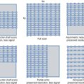
Fig. 3.2
FSE T2 study: comparison of 3.0 T (TR/TE/ETL 4850/81/15, slice thickness 4 mm, FOV 22 cm, matrix 448×320, 2 NEX, 2:39) (a) with 1.5 T (TE/TE/ETL 3000/88/8, slice thickness 6 mm, FOV 24×18, 2 NEX, 256×224, 2:24) (b). At 3.0 T (a) an FSE T2 study takes a similar amount of time as at 1.5 T (b) but achieves greater definition (thinner and more numerous slices, broader matrices and smaller FOV)
3.1.1.2 High Spatial Resolution
SNR is higher at 3 tesla, but the improvement varies with the category of the sequences.
The greater SNR allows increased spatial resolution to be achieved and a reduction of partial volume effects, thereby depicting structures that are difficult to visualize at 1.5 T (e.g. blood vessels measuring 200–300 μm). In addition, the resulting greater spatial resolution makes 3.0 T imaging more accurate when fine morphological detail is required, as in volumetric studies like hippocampal volumetry, which is performed to analyse the extent of hippocampal damage in patients with epilepsy and other diseases involving the brain such as Alzheimer’s [9].
3 T MRI also provides accurate stereotactic data sets [10].
3.1.1.3 High Temporal Resolution
Temporal resolution is also enhanced at higher field intensity due to greatly reduced acquisition time. Indeed, the fast gradients of 3.0 T units allow scanning times to be drastically shortened, resulting in a reduction of motion artefacts.
Using a 3.0 T MR system, morphological investigations of the brain, including a standard high-definition study before and after contrast administration, can be performed in 20–30 min and yield greater detail than using a 1.5 T unit. If diffusion and perfusion studies, spectroscopy and functional MR imaging (fMRI) are also performed, acquisition and processing times do not exceed 50–60 min.
Since intrinsically fast techniques like echoplanar sequences obviously involve similar acquisition times with both low and high field strengths, the greater SNR of the latter is exploited to achieve enhanced spatial resolution (Fig.3.3).

Fig. 3.3
(a–e) SE-EPI (16 shots, matrix 512 × 256). The higher SNR yields greater resolution
High-strength magnetic fields are therefore indicated for fast imaging of patients in poor conditions, for long protocols (including structural, metabolic and functional imaging) and for novel applications such as continuous EEG recording and functional fMRI for the detection of seizure foci [11].
Reduced times of acquisition are also useful with uncooperative and paediatric patients. In the latter, this feature is especially valuable in the case of non-sedated children who may have difficulties in lying still or in sedated neonates in poor conditions: short examination times are thus crucial in both cases [12].
3.1.2 Disadvantages
3.1.2.1 Increased SAR
A major drawback of high magnetic fields is an increased SAR, i.e. the radiofrequency (RF) energy deposited per kilogram of tissue in unit of time. The resonance frequency of the hydrogen protons, hence the RF signal, grows proportionally with magnetic field strength, resulting in more energy being deposited in tissues. As a consequence, the SAR limits are reached sooner with 3.0 T than 1.5 T units, the SAR increasing fourfold from 1.5 T to 3.0 T [13, 14]. Because the SAR increases with the square of the field strength, RF deposition is more limiting at higher field strengths.
Moreover, as the SAR is also proportional to pulse duration and pulse and slice number, its increment at higher magnetic field strengths entails a number of drawbacks, limiting the number of slices, the use of fast spin echo (FSE) sequences, selection of the flip angle (FA) and speed of acquisition. Therefore, sequences such as FSE, which employ a large number of closely spaced RF pulses with large FA, are those most likely to cause increased energy deposition at higher fields and to be affected by SAR level limitations. Unfortunately, as FSE sequences rely on T2- rather than T2*-weighted echo trains, they are the least sensitive to susceptibility-induced image distortion and would be extremely useful at higher magnetic fields.
High magnetic field strength therefore requires a new approach to reduce the SAR, especially when using FSE. Several different strategies have been devised to do this. The most obvious one is to reduce acquisition time via an increase in echo spacing and a reduction in echo train length or by employing partial FA (e.g. 150° instead of 180°). However, these methods impair scanning efficiency (due to longer examination times or to reduced anatomical coverage) or the contrast/noise gain per unit of time. An interesting technique that is not affected by these limitations is the one using hyperechoes, which for tissues with T1>>T2 provides greater signal intensity. Using the hyperecho as the centre k-space line for the image, a greater SNR is achieved with respect to comparable conventional FSE sequences with a marked reduction in SAR.
With T1 sequences, the use of longer TR partially resolves the SAR problem but entails longer imaging times as well as a decrease in the T1 weighting of sequences, which is not necessarily desirable.
By contrast, in gradient echo imaging, lower FA for given TR are used to reduce the SAR. To prevent accidental heating of tissues during scanning, the SAR must always be closely monitored to avoid exceeding the limits laid down by the FDA (Food and Drug Administration) (less than 1 °C in any tissue). This threshold is rarely reached at 1.5 T even using FSE sequences.
Therefore, since sequences can be modified and still yield high-quality images, the SAR is not an insurmountable problem for brain scanning at 3.0 T with the exception of foetal imaging; high-field imagers are thus unlikely to be used for the latter applications in the foreseeable future [12].
The newer MR system designs are inherently more SAR efficient. While the earlier units were so RF intense as to require ‘patient cooling’ intervals between sequences in some cases, the more modern units and their protocols do not normally carry this risk. Limitations in the rate of RF energy deposition continue to place minor restrictions on the number of sections that can be acquired per TR period, thus some of the efficiency gains afforded by the potentially doubled signal intensity of 3.0 T units. The problem is much less severe with newer systems, and section reduction is currently a relatively minor concern also thanks to the increasing diffusion of parallel imaging with multichannel receiver coil arrays, which is becoming an integral part of high-field MR neuroimaging. This technique reduces the effects of SAR by means of a decreased RF exposure achieved by reducing the number of pulses required to obtain a given image with a set resolution. Although this entails an increase in dead time, it is partly offset by the greater SNR of 3.0 T systems. For this reason, high-field imaging is the ideal platform for parallel imaging because it helps to offset the low SNR of parallel imaging.
3.1.2.2 Increased Acoustic Noise
The acoustic noise generated by rapid gradient switching within the main magnetic field, which increases with field strength, is another considerable disadvantage of 3.0 T units. The noise is twice that generated in a 1.5 T MR system and may exceed 119 dB, especially with fast sequences like fast SE, fast gradient echo (FGE) and echoplanar imaging (EPI). However, this disadvantage can also be overcome relatively easily by using parallel imaging.
3.1.2.3 Dielectric Resonance Effect
This phenomenon is connected with the distortion of the B 1 field by the body of the subject in the tunnel when volume coils are used at high fields. In particular, as the field strength, and therefore the Larmor frequency, increases – while the wavelength decreases – body size becomes significant with respect to the wavelength of the radiation transmitted, particularly in the presence of a high dielectric constant of the body. This results in a change in the intensity of the signal, which will often exhibit a bright centre and relatively hypointense borders [17, 18].
3.2 Diagnostic Features of 3.0 T MR Imaging
The main differences compared with lower-field strength systems are (1) changes in tissue contrast, (2) increased magnetic susceptibility and (3) increased chemical shift.
3.2.1 Changes in Tissue Contrast
Whereas proton density is clearly a magnetic field-independent parameter, T1 and T2 relaxation times are field dependent, usually increasing and, respectively, decreasing at higher magnetic fields.
The rates at which excited protons relax are a function of magnetic field strength. In general, the longitudinal or spin-lattice relaxation rate (R1 = 1/T1) of certain tissues (e.g. semisolids) decreases with field strength, whereas the transverse relaxation rate (R2 = 1/T2) is scarcely affected [5, 19]. This leads to a 25–40 % increase in T1 relaxation time in tissues on passing from 1.5 T to 3.0 T fields. By contrast, for biological fluids (like CSF and blood), the longitudinal rate is weakly affected, so that R1 and R2 are basically equal at both field intensities. As a result, given the same TR, T1 weighting is greater at 3.0 T than at 1.5 T. Good T1 contrast can also be achieved using relatively long TR.
The increase in T1 relaxation time is a major drawback in high-field SE T1 imaging, as the reduction in T1 differences between tissues results in loss of contrast (Fig. 3.4).

Fig. 3.4
T1 imaging: SE T1 sequence acquired at 3.0 T (TR/TE 500/min, slice thickness 5 mm, FOV 24, matrix 320×224, 1 NEX, 2:00) (a) and 1.5 T (TR/TE 500/min, slice thickness 5 mm, FOV 24 cm, matrix 256×192, 1 NEX, 1:23) (b). The increased T1 involves reduced contrast at 3.0 T with respect to 1.5 T
T1 lengthening with increasing magnetic field also applies to blood. Blood T1 is insensitive to the level of oxygenation and increases linearly with field strength. This is particularly valuable in MR angiography (especially in time-of-flight sequences), as it involves greater background suppression due to a lower R1 of stationary tissues and a greater flow enhancement given the broadly constant R1 of blood, thus yielding better vessel-tissue contrast (Fig. 3.5) [20, 21].

Fig. 3.5


Normal arterial circulation: 3D TOF study at 3.0 T (a) and 1.5 T (b). Vascular conspicuity and background are greater in (a) (TOF SPGR TE/TE/FA 30/min/20, slice thickness 1.4 mm, matrix 512×320, ZIP 1024, ZIP 2, 1 NEX, 50 locations per slab, 6:18) than in (b) (TOF SPGR TE/TE/FA 45/4/20, slice thickness 1.4 mm, FOV 24×18, matrix 512×224, 1 NEX, 50 locations per slab, 6:22) resulting in greater vessel-tissue contrast
Related posts:
Stay updated, free articles. Join our Telegram channel
Full access? Get Clinical Tree
