Adaptive Noise Reduction and Edge Enhancement in Medical Images by Using ICA

(13.1)

where A is an unknown mixing matrix. In the application of ICA to feature extraction, the columns of A represent the basis functions and s _irepresent the i-th feature in the observed data x. The aim of ICA is to find a matrix W, such that the resulting vector

$\displaystyle{ {\bf y} = {\bf Wx} }$

(13.2)

recovers the independent sources s, with its probability permuted and rescaled. Each row of W is taken as a filter. To obtain a more unique solution, s _iis usually assumed to have unit variance.

Contrary to PCA, the basis functions of ICA cannot be analytically calculated. The adopted method involves minimizing or maximizing some relevant criterion functions. Several ICA algorithms have been proposed, one of which and its detail implementation will be introduced in section “Basis Functions Learned by ICA”.

Before performing ICA, the problem associated with estimating the matrix A can be simplified by a prewhitening of the data x. The observed vector x is first linearly transformed into a vector

$\displaystyle{ {\bf z} = {\bf M}{\bf x} }$

(13.3)

whose correlation matrix equals unity: E{zz ^T} = I. This can be accomplished by PCA with

$\displaystyle{ {\bf M} ={ {\bf D}}^{-1/2}{\bf V} }$

(13.4)

where the matrix V is the eigenvector matrix and D is the corresponding eigenvalue matrix. At the same time, the dimensionality of the data is reduced. After this transformation, we have

$\displaystyle{ {\bf z} = {\bf Mx} = {\bf MAs} = {\bf Bs} }$

(13.5)

where the matrix B is the mixing matrix. ICA is performed on the sphered data z and the estimated mixing matrix B is an orthogonal matrix because $E\{{{\bf zz}}^{T}\} = {\bf B}E\{{{\bf ss}}^{T}\}{{\bf B}}^{T} ={ {\bf BB}}^{T} = {\bf I}$ . The basis function matrix A of the original data x is

$\displaystyle{ {\bf A} ={ {\bf V}}^{T}{{\bf D}}^{1/2}{\bf B} }$

(13.6)

Figure 13.1 presents an example of two non-Gaussian (super-Gaussian) distributed sources (Fig. 13.1a) and the scatter (Fig. 13.1b) of their mixed variables. The basis functions obtained by PCA and ICA are also plotted in Fig. 13.1b, which confirms that PCA transformation cannot capture the main structure of non-Gaussian data. However, ICA can precisely determine the directions of the inherent data structure by maximizing independence.

Fig. 13.1

PCA and ICA transformations. (a) two components of super-Gaussian data, (b) the scatter of the data, and the obtained ICA and PCA basis functions of (a)

Image Model

An image patch x from an image I can be represented by a linear combination of basis functions as in (13.7), where A _i(size: N’ by 1, N’ is the dimension of x) is the ith basis function and y _iare the coefficients, which can be used as image features or image coding. Unlike the Fourier transform or wavelet-based methods, in our proposed ICA-based method, the basis functions are learned by ICA from similar structure images with processing images. The advantage of ICA-based method is that we can obtain a set of adaptive basis functions based on images alone.

$\displaystyle{ {\bf x} = {\bf Ay} =\sum _{ i=0}^{N-1}{\bf A}_{ i}\mathit{y}_{i} = {\bf A}_{0}\mathit{y}_{0} + {\bf A}_{1}\mathit{y}_{1} + {\bf A}_{2}\mathit{y}_{2} + \cdots + {\bf A}_{N-1}y_{N-1} }$

(13.7)

Basis Functions Learned by ICA

In (13.7), we attempt to obtain A using ICA (size: N’ by N, N is the number of ICA basis functions. In our experiments, we retained N’ basis functions in ICA learning: i.e., N’=N) ) from sample image x only, which can also be viewed as a Blind Source Separation (BSS) problem, and can be solved by ICA [10]. The aim of BSS is to find a matrix W, called a separator, that results in the estimates of the coefficients of y to be as statistically independent as possible for a set of data (x), as shown in (13.2)

$\displaystyle{ {\bf y} = {\bf W}{\bf x} }$

(13.8)

The estimates or independent components y may be permuted and rescaled. The ICA transformation matrix W (size: N by N) can be calculated as: W=A ⁻¹. For the reasons given in [18], we orthogonalize W by ${\bf W} = {\bf W}{({{\bf W}}^{T}{\bf W})}^{-1/2}$ , and A and W then become square unitary matrices with each row corresponding to a basis function (amounting to a column of mixed matrix A under the condition of orthogonalized W. In our method, we need to reconstruct images, hence the basis that is used should be orthogonalized and integrated as with the Fourier and wavelet basis).

Bell and Sejnowski proposed a neural learning algorithm for ICA [14, 15]. This approach employs the maximization of the joint entropy by using a stochastic gradient ascent. The updating formula for W is

$\displaystyle{ \Delta {\bf W} = ({\bf I} + g({\bf y}){{\bf y}}^{T}){\bf W}, }$

(13.9)

where y = W x and $g({\bf y}) = {\bf 1} -{\bf 2}/({\bf 1} + {e}^{-{\bf y}})$ is calculated for each component of y. Before the learning procedure, x is sphered by subtracting the mean and multiplying by a whitening filter ${\bf W}_{0} = [({\bf x} - E({\bf x}))({\bf x} -{ E({\bf x}))}^{T}{]}^{-1/2}$ :

$\displaystyle{ {\bf x}_{0} = {\bf W}_{0}({\bf x} - E({\bf x})), }$

(13.10)

where x ₀ the whitening data. The aim of the whitening (standardization) by using W ₀ is to make the mixture and separator unitary. Therefore, the complete transform is calculated as the product of the whitening matrix and learned matrix:

$\displaystyle{ {\bf W}_{I} = {\bf W}{\bf W}_{0}. }$

(13.11)

To extract the adaptive basis functions by using ICA for image representation, we have to prepare training samples using images that are similar to processed data. In our experiment, more than 10,000 image patches are usually randomly selected as training data samples, which from our experience will be sufficient to obtain reliable basis functions of training images. At the same time, it will not be sufficient for learning over a long time period. The learned ICA basis functions by using natural images are shown in Fig. 13.2. The patch size of each image sample is set as 8 ×8 and an example regarding the formation of the observation vectors from images is shown in Fig. 13.3.

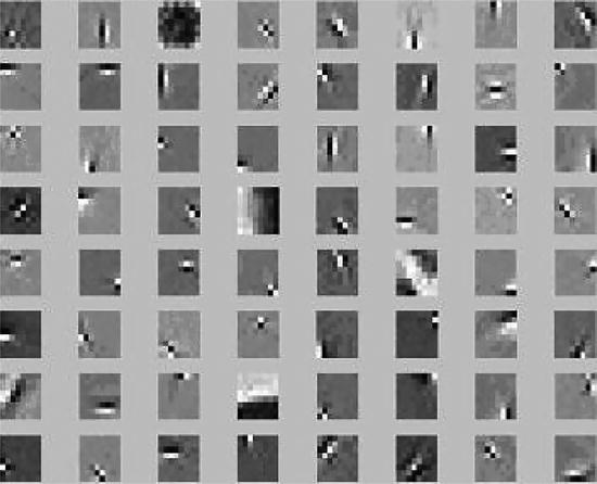
Fig. 13.2

The ICA basis functions obtained using natural images as training samples

Fig. 13.3

The ICA input observation vector obtained from one sample patch

Adaptive Noise Reduction for PET Images

PET is one of the most important tools for medical diagnostics that has been recently developed. Projection data in PET are acquired as the number of photon counts from different observation angles [13, 25]. Positron decay is a random phenomenon that causes undesirable high variations in measured sinograms, which appear as quantum noise [26]. The reduction of quantum noise or Poisson noise in medical images is an important issue because the quantum noise usually obeys a Poisson law; therefore, it is highly dependent on the underlying intensity pattern being imaged. The contaminated image can therefore be decomposed as the true mean intensity and Poisson noise, and the noise represents the variability of the pixel amplitude about the true mean intensity [27]. It is well known that the variance of a Poisson random variable is equal to the mean: σ ² = u. Then, the SNR for an image with a Poisson image is given by

$\displaystyle{ SNR = \frac{u} {\sigma } = \frac{u} {\sqrt{{\sigma }^{2}}} = \frac{u} {\sqrt{u}} = \sqrt{u} }$

(13.12)

Thus, the variability of the noise is proportional to the intensity of the image and is therefore signal dependent [23]. This signal dependence makes it much more difficult to separate the signal from noise. The current methods for Poisson noise reduction include mainly two types of strategies. One would be to work with the square root of a noisy image because the square root operation is a variance stabilizing transformation. However, after preprocessing, Poisson noise will not tend to be a white noise if there are only a few photons present. Thus, it is not entirely suitable to adopt the Gaussian noise reduction algorithm. The other strategy is the method of wavelet shrinkage. However, the basic functions of wavelet transformation are fixed and cannot adapt to different types of sets. In this chapter, we explain the development of an adaptive noise reduction strategy called the ICA-based filter, in the sinogram domain for PET. The shrinkage scheme (filter) adapts to both signal and noise and balances the trade-off between noise removal and excessive smoothing of image details. The filtering procedure has a simple interpretation as a joint edge detection/estimation process. Our method is closely related to the method of wavelet shrinkage; however, compared with other wavelet methods, it has an important benefit that the representation is solely determined by the statistical properties of the data sets. Therefore, ICA-based methods will perform better than the wavelet-based Poisson noise reduction method in denoising applications. At the same time, we also compared the denoising results of different ICA basis functions that are trained from different data sets.

ICA-Based Shrinkage Algorithm

Shrinkage is an increasingly popular method in the wavelet domain for curve and surface estimation. The wavelet shrinkage procedure for statistical applications was developed by Donoho [28]. This shrinkage method relies on the basic idea that the energy of a signal (that is partially smoothed) will often be concentrated within a few coefficients in the wavelet domain, whereas the noise energy is spread among all coefficients. Therefore, the shrinkage function in the wavelet domain will tend to retain a few larger coefficients that represent the signal, whereas the noise coefficients will tend to reduce to zero.

In image decomposition by using ICA, the extracted basis functions represent different properties of training images and those representing clear image information will be almost sparse [21]. Thus, the energy of clear image information will be concentrated in a few coefficients of the ICA components. However, if noise is projected to the ICA basis functions, the energy will uniformly spread in the ICA domain. Hence using the shrinkage method in the ICA domain, we can remove noise in a similar manner as in the wavelet shrinkage procedure.

We assume that an observe an n-dimensional vector is contaminated by noise. We denote the observed noisy vector as x, the original non-Gaussian vector as P, and the noise signal as v. We then have

$\displaystyle{ {\bf x} = {\bf P} + {\bf v} }$

(13.13)

The goal of signal denoising is to find P ^′ = g ^′(x) such that P ^′is close to P in some well-defined sense. The following gives the ICA-based shrinkage procedure:

Step 1

Estimate an orthogonal ICA transformation matrix W by using the training data (the observed data x or a set of representative data z).

Step 2

For the observed data x (corrupted by noise), use the ICA transformation matrix W to transform into ICA-domain components:

$\displaystyle{ {\bf y} = {\bf W}{\bf x} }$

(13.14)

where y can be considered to be a sparse variable, which is also corrupted by noise.

Step 3

Use the ICA-based shrinkage method to estimate noise-free components y ^′for the noisy variable y:

$\displaystyle{{ {\bf y}}^{^{\prime}}_{i} = g_{i}({\bf y}_{i}) }$

(13.15)

Step 4

Invert the denoised variable y ^′and get an estimation of original data P:

$\displaystyle{{ {\bf P}}^{^{\prime}} = {\bf A}{{\bf y}}^{^{\prime}} }$

(13.16)

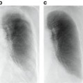
where ${\bf A} = [{\bf A}_{0},{\bf A}_{1},\cdots ,{\bf A}_{N-1}] = {[{\bf W}_{0}^{T},{\bf W}_{1}^{T},\cdots ,{\bf W}_{N-1}^{T}]}^{T}$ are the ICA basis functions.

In step (3), g(y) is the operator or function of the shrinkage and is used to reduce the noise. In PET images, the noise is signal-dependent Poisson noise; hence, we mainly aim to reduce Poisson noise in the images. In the next subsection, based on Poisson noise’s special property, we present an efficient shrinkage scheme with the adaptive ICA basis functions, which can be obtained directly from noisy data, as shown in Fig. 13.4 for PET images. In addition, we select some clean natural images and processed data (observed data) as the training data to estimate the ICA basis functions, and then apply two sets of the ICA basis functions (as shown in Fig. 13.2) to the denoising procedure for comparison purposes. The flowchart of the ICA-based filter for actual PET sinograms is shown in Fig. 13.5.

Fig. 13.4

The ICA basis functions obtained using actual PET images as training samples

Fig. 13.5

Flowchart of the ICA-based noise reduction strategy using two sets of learned basis functions from natural and PET images, respectively

ICA Based Filter for Poisson Noise

In our previous work [17, 18], we proposed a shrinkage function based on the cross-validation algorithm [14] for Poisson noise. The shrinkage function g(y) is given by [17]

$\displaystyle{ g({\bf y}) ={ {\bf y}}^{^{\prime}} = {\bf y}\frac{{{\bf y}}^{2} {-\boldsymbol{ \sigma }}^{2}} {{{\bf y}}^{2}} }$

(13.17)

where σ ² is the power of Poisson noise. The noise power of the ith component with ICA basis functions trained from clean natural images can be estimated by [20]

$\displaystyle{{ \sigma _{i}}^{2} = ({\bf W}_{ i}. {\ast}{\bf W}_{i}){\bf x} }$

(13.18)

where the symbol of “.*” represents the multiplication of each entry in vector 1 with its corresponding entry in vector 2, W _iis the ith row of the ICA transformation matrix W(the ith ICA basis function), and σ _i² represents the ith noisy power component in the ICA domain(a row of samples). For clean natural images as the training set, the obtained ICA transform matrix W can be considered as a local directional filters. The components obtained by ICA transformation would then be the inner product of the image patch and local filters W _i(which is needed to reshape the row vector W _iinto an l

Only gold members can continue reading. Log In or Register to continue