Fig. 9.1
Illustration of (a) an original standard chest radiograph and (b) the corresponding VDE soft-tissue image by use of our original MTANN method
The purpose of this study was to separate rib edges, ribs close to the lung wall, and clavicles from soft tissue in CXRs. To achieve this goal, we newly developed anatomically (location-) specific multiple MTANNs, each of which was designed to process the corresponding anatomic segment in the lungs. A composite VDE bone image was formed from multiple output images of the anatomically specific multiple MTANNs by using anatomic segment masks, which were automatically segmented. In order to make the contrast and density of the output image of each set of MTANNs consistent, histogram matching was applied to process the training images. Before a VDE bone image was subtracted from the corresponding CXR to produce a VDE soft image, a total variation (TV) minimization smoothing method was applied to maintain rib edges. Our newly developed MTANNs were compared with our conventional MTANNs.
Methods
Database
The database used in this study consisted of 119 posterior–anterior CXRs acquired with a computed radiography (CR) system with a dual-energy subtraction unit (FCR 9501 ES; Fujifilm Medical Systems, Stamford, CT) at The University of Chicago Medical Center. The dual-energy subtraction unit employed a single-shot dual-energy subtraction technique, where image acquisition is performed with a single exposure that is detected by two receptor plates separated by a filter for obtaining images at two different energy levels [29–31]. The CXRs included 118 abnormal cases with pulmonary nodules and a “normal” case (i.e., a nodule-free case). Among them, eight nodule cases and the normal case were used as a training set, and the rest were used as a test set. The matrix size of the chest images was 1,760 × 1,760 pixels (pixel size, 0.2 mm; grayscale, 10 bits). The absence and presence of nodules in the CXRs were confirmed through CT examinations. Most nodules overlapped with ribs and/or clavicles in CXRs.
Multi-Resolution MTANNs for Bone Suppression
For bone suppression, the MTANN [32] consisted of a machine-learning regression model such as a linear-output multilayer ANN regression model [33], which is capable of operating directly on pixel data. This model employs a linear function instead of a sigmoid function as the activation function of the unit in the output layer. This was used because the characteristics of an ANN have been shown to be significantly improved with a linear function when applied to the continuous mapping of values in image processing [33, 34]. Other machine-learning regression models can be used in the MTANN framework (a.k.a., pixel-based machine learning [25]) such as support vector regression and nonlinear Gaussian process regression models [35]. The output is a continuous value.
The MTANN involves training with massive subregion-pixel pairs which we call a massive-subregions training scheme. For bone suppression, CXRs are divided pixel by pixel into a large number of overlapping subregions (or image patches). Single pixels corresponding to the input subregions are extracted from the teaching images as teaching values. The MTANN is massively trained by using each of a large number of the input subregions (or patches) together with each of the corresponding teaching single pixels. The inputs to the MTANN are pixel values in a subregion (or an image patch), R, extracted from an input image. The output of the MTANN is a continuous scalar value, which is associated with the center pixel in the subregion, represented by
where ML(·) is the output of the machine-learning regression model, and I(x,y) is a pixel value of the input image. The error to be minimized by training of the MTANN is represented by
where c is the training case number, O c is the output of the MTANN for the cth case, T c is the teaching value for the MTANN for the cth case, and P is the number of total training pixels in the training region for the MTANN, R T .
(9.1)
(9.2)
Bones such as ribs and clavicles in CXRs include various spatial-frequency components. For a single MTANN, suppression of ribs containing such variations is difficult, because the capability of a single MTANN is limited, i.e., the capability depends on the size of the subregion of the MTANN. In order to overcome this issue, multi-resolution decomposition/composition techniques were applied.
First, input CXRs and the corresponding teaching bone images were decomposed into sets of images of different resolution and these were then used for training three MTANNs in the multi-resolution MTANN. Each MTANN is an expert for a certain resolution, i.e., a low-resolution MTANN is responsible for low-frequency components of ribs, a medium-resolution MTANN is for medium-frequency components, and a high-resolution MTANN for high-frequency components. Each resolution MTANN is trained independently with the corresponding resolution images. After training, the MTANNs produce images of different resolution, and then these images are combined to provide a complete high-resolution image by use of the multi-resolution composition technique. The complete high-resolution image is expected to be similar to the teaching bone image; therefore, the multi-resolution MTANN would provide a VDE bone image in which ribs are separated from soft tissues.
Anatomically (Location-) Specific Multiple MTANNs
Although an MTANN was able to suppress ribs in CXRs [23], the single MTANN did not efficiently suppress rib edges, ribs close to the lung wall, and the clavicles, because the orientation, width, contrast, and density of bones are different from location to location, and because the capability of a single MTANN is limited. To improve the suppression of bones at different locations, we extended the capability of a single MTANN and developed an anatomically specific multiple-MTANN scheme that consisted of eight MTANNs arranged in parallel, as shown in Fig. 9.2a. Each anatomically specific MTANN was trained independently by use of normal cases and nodule cases in which nodules were located in the corresponding anatomic segment. The lung field was divided into eight anatomic segments: a left-upper segment for suppression of left clavicles and ribs, a left hilar segment for suppression of bone in the hilar area, a left middle segment for suppression of ribs in the middle of the lung field, a left lower segment for suppression of ribs in the left lower lobe, a right upper segment, a right hilar segment, a right middle segment, and a right lower segment. For each anatomically specific MTANN, the training samples were extracted specifically from the corresponding anatomic segment mask (the training region in Eq. 9.2).
Fig. 9.2
Architecture and training of our new anatomically specific MTANNs. (a) Training phase. (b) Execution phase
After training, each of the segments in a non-training CXR was inputted into the corresponding trained anatomically specific MTANN for processing of the anatomic segment in the lung field, e.g., MTANNs No. 1 was trained to process the left-upper segment in the lung field in which the clavicle lies; MTANNs No. 2 was trained to process the left hilar segment, etc., as illustrated in Fig. 9.2b. The eight segmental output sub-images from the anatomically specific multiple MTANNs were then composited to an entire VDE bone image by use of the eight anatomic segment masks. To blend the sub-images smoothly near their boundaries, anatomic segmentation masks smoothed by a Gaussian filter were used to composite the output sub-images, represented by
![$$ {f}_b\left(x,y\right)={\displaystyle \sum_{i=1}^8{O}_i\left(x,y\right)\times {f}_G\left[{M}_i\left(x,y\right)\right]}, $$](/wp-content/uploads/2016/03/A218098_1_En_9_Chapter_Equ3.gif)
where f b (x,y) is the composite bone image, O i is the ith trained anatomically specific MTANN, f G (·) is a Gaussian filtering operator, and M i is the ith anatomic segmentation mask.
(9.3)
Training Method
In order to make the output image of each set of anatomical segment MTANNs consistent in density and contrast, it is preferable to use similar CXRs to train each anatomical segment. A normal case was therefore selected for training the eight MTANNs with different segments of the lung field. In order to maintain nodule contrast while suppressing bone structures, nodule cases were used to train the anatomical segment-specific multiple MTANNs as well. As it is impossible to find an abnormal case where each of eight typical nodules is located in each of the eight anatomical segments in the lung field, eight different nodule cases were required for training eight anatomical MTANNs. For each nodule case, a nodule was located in the anatomical segment that was used to train the corresponding MTANN. As a result, nine CXRs were used, i.e., one normal case and eight nodule cases, along with the corresponding dual-energy bone images for training the eight sets of multi-resolution MTANNs.
For training of overall features in each anatomic segment in the lung field, 10,000 pairs of training samples were extracted randomly from the anatomic segment for each anatomically specific MTANN: 5,000 samples from the normal case; and 5,000 samples from the corresponding nodule case. A three-layered MTANN was used, where the numbers of input, hidden, and output units were 81, 20, and 1, respectively. Once the MTANNs are trained, the dual-energy imaging system is no longer necessary. The trained MTANNs can be applied to standard CXRs for suppression of bones; thus, the term “virtual dual-energy” (VDE) technology. The advantages of this technology over real dual-energy imaging are that there is no need for special equipment to produce dual-energy images, or no additional radiation dose to patients.
Because of differences in acquisition conditions and patients among different CXRs, the density and contrast vary within the different training images. This makes the training of the eight anatomically specific MTANNs inconsistent. To address this issue, a histogram-matching technique was applied to training images to equalize the density and contrast. Histogram matching is a technique for matching the histogram of a given image with that of a reference images. We used a normal case as the reference image to adjust the nodule cases. First the cumulative histogram F 1 of the given image and that F 2 of the reference image were calculated. Then, the histogram transfer function M(G 1 ) = G 2 was calculated so that F 1 (G 1 ) = F 2 (G 2 ). Finally, the histogram transfer function M was applied to each pixel in the given image.
The proportion of background also varies among different CXRs. The histogram matching of an image with a larger proportion of the background to another with a small proportion may cause the density of the lung field in the matched image to appear darker than the target image. For this reason, only the histogram of the body without the background was matched in the target image. The background was first segmented, which typically corresponds to the highest signal levels in the image where the unobstructed radiation hits the imaging plate. Several factors make the detection of these regions a challenging task. First, the radiation field across the image may be nonuniform due to the orientation of the X-ray source relative to the imaging plate, and the effect of scatter in thicker anatomical regions compounds this problem. Further, for some examinations, multiple exposures may be carried out on a single plate, resulting in multiple background levels. The noise attributes of the imaging system were used to determine if the variation around a candidate background pixel is a typical range of direct exposure pixel values. The corresponding values of candidate background pixels were accumulated in a histogram, and the resulting distribution of background pixel values invariably contained well-defined peaks, which served as markers for selecting the background threshold. After analyzing the histogram, the intensity values to the left of the background peak clearly represented the background, while those to the right represented, to a progressively greater extent, the intensity values of image information. The portion of the histogram to the right of the background peak was processed to find the point at which the histogram first exhibited a change in its curvature from negative to positive. For an increase in intensity, a negative curvature corresponds to a decreasing rate of occurrence of background pixels, while a positive curvature corresponds to an increasing rate of occurrence. In this manner, it was possible to create a difference histogram to obtain a positive slope at the intensity position to the right of the background peak. At this position, we could determine the counts for the least intense pixels, whose intensities are mostly due to the signal. After finding the intensity level representative of the minimum signal intensity level, this level was applied as a signal threshold for segmenting the background. This approach successfully dealt with the problems of non-uniform backgrounds. Figure 9.3 illustrates our background segmentation. A background peak is seen in the histogram illustrated in Fig. 9.3a. Figure 9.3c illustrates a segmentation threshold determined by finding the right bin to the background peak in the difference histogram. Figure 9.3d shows the background segmentation result by using the threshold value.
Fig. 9.3
Background segmentation. (a) Histogram of pixel values in CXR (b). (b) Original CXR. (c) Differences between two neighboring bins in histogram (a). (d) Background segmentation result
Automated Anatomic Segmentation
To train and process anatomically specific MTANNs, a given CXR was divided into anatomic segments. Each segment was inputted into each of anatomically specific MTANNs simultaneously. Each MTANN provided the corresponding segment of a VDE bone image where bones were extracted. Because each MTANN is an expert for a specific anatomic segment, the signal-to-noise ratio is highest in the corresponding anatomic segment among all segments, as illustrated in Fig. 9.4. Merging all anatomic segments provided a complete single VDE bone image where the signal-to-noise ratio is high in all segments.
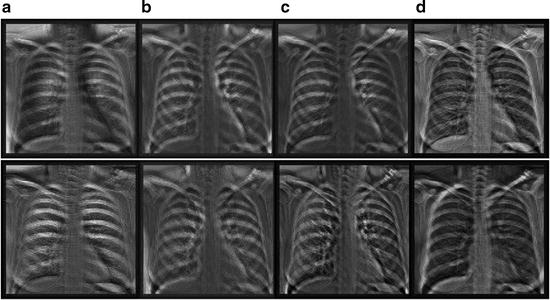
Fig. 9.4
Eight output bone images of the trained anatomically specific multiple MTANNs. (a) Output from the segment MTANNs trained for the hilar region, (b) Output from the MTANNs trained for the lower region of the lung, (c) Output from the MTANNs trained for the middle region of the lung, (d) Output from the MTANNs trained for the upper region of the lung
To determine eight anatomic segments, an automated anatomic segmentation method was developed based on active shape models (ASMs) [36]. First, the lung fields were segmented automatically by using a multi-segment ASM (M-ASM) scheme [37], which can be adapted to each of the segments of the lung boundaries (which we call a multi-segment adaptation approach), as illustrated in Fig. 9.5. As the nodes in the conventional ASM are equally spaced along the entire lung shape, they do not fit parts with high curvatures. In our developed method, the model was improved by the fixation of selected nodes at specific structural boundaries that we call transitional landmarks. Transitional landmarks identified the change from one boundary type (e.g., a boundary between the lung field and the heart) to another (e.g., a boundary between the lung field and the diaphragm). This resulted in multiple segmented lung field boundaries where each segment is correlated with a specific boundary type (heart, aorta, rib cage, diaphragm, etc.). The node-specific ASM was built by using a fixed set of equally spaced nodes for each boundary segment. Our lung M-ASM consisted of a total of 50 nodes for each lung boundary that were not equally spaced along the entire contour. A fixed number of nodes were assigned to each boundary segment, and they were equally spaced along each boundary (as shown in Fig. 9.5). For example, the boundary between the left lung field and the heart consisted of 11 points in every image, regardless of the actual extent of this boundary in the image (see Fig. 9.5). This allowed the local features of nodes to fit a specific boundary segment rather than the whole lung, resulting in a marked improvement in the accuracy of boundary segmentation. From the training images, the relative spatial relationships among the nodes in each boundary segment were learned in order to form the shape model. The nodes were arranged into a vector x and projected into the principal component shape space, represented by the following equation:
where V = (V 1 V 2 …V M ) is the matrix of the first M eigenvectors for the shape covariance matrix, and b = (b 1 b 2 …b M ) T is a vector of shape coefficients for the primary axes. The shape coefficients were constrained to lie in a range  to generate only a plausible shape and projected back to node coordinates, represented by:

where m usually has a value between 2 and 3 [38], and was 2.5 in our experiment.
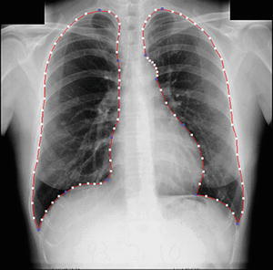
Fig. 9.5
Lung segmentation using our M-ASM. Blue points represent the transitional landmarks of two boundary types
(9.4)
to generate only a plausible shape and projected back to node coordinates, represented by:(9.5)
After the lungs were segmented, they were automatically divided into eight anatomic segments by using the boundary types and the transitional landmarks. By using the landmark points, we obtained the upper region, lower region, and hilar region in each lung, as illustrated in Fig. 9.6. The eight output segmental images from the multiple MTANNs were merged into a single VDE bone image:
where f i b (x,y) is the output image from the i–th MTANN and m i b (x,y
 Computational Intelligent Image Analysis for Assisting Radiation Oncologists’ Decision Making in Radiation Treatment Planning
 The Role of Content-Based Image Retrieval in Mammography CAD
 Liver Volumetry in MRI by Using Fast Marching Algorithm Coupled with 3D Geodesic Active Contour Segmentation
 Computational Anatomy in the Abdomen: Automated Multi-Organ and Tumor Analysis from Computed Tomography
 Subtraction Techniques for CT and DSA and Automated Detection of Lung Nodules in 3D CT
 Image Segmentation for Connectomics Using Machine Learning


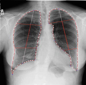
Fig. 9.6
Result of automated anatomic segmentation based on our M-ASM
(9.6)
Related posts:
Computational Intelligent Image Analysis for Assisting Radiation Oncologists’ Decision Making in Radiation Treatment Planning
The Role of Content-Based Image Retrieval in Mammography CAD
Liver Volumetry in MRI by Using Fast Marching Algorithm Coupled with 3D Geodesic Active Contour Segmentation
Computational Anatomy in the Abdomen: Automated Multi-Organ and Tumor Analysis from Computed Tomography
Subtraction Techniques for CT and DSA and Automated Detection of Lung Nodules in 3D CT
Image Segmentation for Connectomics Using Machine Learning
Stay updated, free articles. Join our Telegram channel
Full access? Get Clinical Tree
