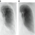
Fig. 10.1
Left: Two ssTEM sections from the Drosophila first instar larva VNC [8]. Right: Corresponding ground truth maps for cell membranes (black). Data: Cardona Lab, ETH
The supervised learning strategy for connectomics has its own challenges that need to be addressed. First, generating training data from electron microscopy images can be a cumbersome task for humans. On the other hand, no training data is needed for deterministic approaches. Second, the training set can be extremely large since each pixel in the training image becomes a training example. This requires a lengthy training stage. In comparison, no training time is spent in deterministic approaches. Third, overfitting is a possibility as in any machine learning application. Finally, the cell membrane classification step demands extremely high accuracy. Even with high pixel accuracy rates such as 95 %, which is acceptable in many other applications, it is virtually certain that almost every neuron in a volume will be incorrectly segmented due to their global, tree-like structure, and correspondingly large surface area. The lack of reliable automated solutions to these problems is the current bottleneck in the field of connectomics. In this chapter, we will describe our approach to deal with each of these problems.
Background
Connectomics from Electron Microscopy
Compared with other imaging techniques, such as MRI [15] and scanning confocal light microscopy [16–20], electron microscopy provides much higher resolution and remains the primary tool for connectomics. The only complete reconstruction of a nervous system to date has been performed for the nematode Caenorhabditis elegans (C. elegans) which has 302 neurons and just over 6,000 synapses [21–23]. This reconstruction, performed manually, is reported to have taken more than a decade [4]. Recently, high throughput serial section transmission electron microscopy (ssTEM) [5, 6, 9, 24–26] and serial block-face scanning electron microscopy (SBFSEM) [4, 10, 27] have emerged as automated acquisition strategies for connectomics. Automatic Tape-Collecting Lathe Ultramicrotome (ATLUM) [28] is another promising technology for speeding up data collection for connectomics.
In the ssTEM technique, sections are cut from a specimen block and suspended so that an electron beam can pass through it, creating a projection which can be captured digitally or on film with 2 nm in-plane resolution. This extremely high resolution is sufficient for identifying synapses visually. An important trade-off occurs with respect to the section thickness: thinner sections, e.g. 30 nm, are easier to analyze because structures are crisper due to less averaging whereas thicker sections, e.g. 90 nm, are easier to handle physically without loss. Through mosaicking of many individual images [29, 30], ssTEM offers a relatively wide field of view to identify large sets of cells as they progress through the sections. Image registration techniques are necessary to align the sections into a 3D volume [6, 31].
In the SBFSEM technique, sections are cut away, and the electron beam is scanned over the remaining block face to produce electron backscatter images. Since the dimensions of the solid block remain relatively stable after sectioning, there is no need for image registration between sections. However, the in-plane resolution is closer to 10 nm which is a disadvantage compared to ssTEM. Typical section thicknesses for SBFSEM are 30–50 nm.
New projects using the techniques described above capture very large volumes containing several orders of magnitude more neurons than the C. elegans. As an example, Fig. 10.2 shows two mosaic sections from a 16 TB ssTEM retina volume [32] that was assembled with our algorithms [6, 31]. It is not feasible to reconstruct complete neural circuits in these datasets with manual methods. Moreover, population or screening studies are unfeasible since fully manual segmentation and analysis would require years of manual effort per specimen. As a result, automation of the computational reconstruction process is critical for the study of these systems.
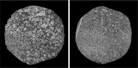
Fig. 10.2
Two sections from the retinal connectome [32] which comprises 341 sections. Each section is ∼ 32 GB and comprises 1,000 image tiles, each 4, 096 ×4, 096 pixels. The circular area with data is approximately 132, 000 pixels in diameter. The complete dataset is ∼ 16 TB. Data: Marc Lab, University of Utah
Finally, as an alternative to SBFSEM and ssTEM, fully 3D approaches such as focused ion-beam scanning electron microscopy (FIBSEM) [33] and electron tomography [34–36] produce nearly isotropic datasets. Both techniques are limited to studying small volumes which is a disadvantage for their use for connectomics. FIBSEM uses a focused-ion beam to mill away sections instead of cutting sections with a knife. While it is clear that these datasets are easier to analyze accurately, the amount of data and the time it would take to acquire and analyze them is prohibitive for large-scale circuit reconstruction applications for the time being.
Neuron Segmentation
Figure 10.2b shows the complexity of the problem. This image which is 132, 000 pixels in diameter contains thousands of neuronal processes. The larger structures seen in Fig. 10.2a are the cell bodies of these processes. Reconstructing neural circuits from EM datasets involves segmenting individual neurons in 3D and finding the synapses between them. Neuron segmentation is the immediate challenge and thus has gathered significantly more attention than synapse detection. The only successful automatic synapse detection approaches so far have been limited to FIBSEM data which offers almost isotropic resolution [37]. In this chapter, we limit our attention to neuron segmentation. There are two general strategies for neuron segmentation. One strategy is to directly segment neurons in 3D [38, 39]. However, this can be difficult in many datasets due to the anisotropic nature of the data. The large section thickness often causes features to shift significantly between sequential images both in ssTEM and SBFSEM, decreasing the potential advantages of a direct 3D approach. The other strategy first segments neurons in two-dimensional (2D) images followed by linking them across sections to form a complete neuron [40–43]. Our approach fits in this second category. In this chapter, we focus on the 2D neuron segmentation problem. For linking 2D neuron regions across sections we refer the reader to [41, 44–46].
Image Processing Methods
Neuron segmentation has been studied mostly using semi-automated methods [8, 24, 40, 43, 47]. Fully automatic segmentation is complicated by two main challenges: complex intracellular structures such as vesicles and mitochondria that are present in the ssTEM images and the extremely anisotropic resolution of the data, e.g. 2 nm in-plane vs. 40 nm out-of-plane. Previous automatic EM segmentation methods include active contours which rely on an gradient term to drive the segmentation [42, 48–53]. This gradient/edge term can be ambiguous because of the locally similar appearance of neuron and intracellular membranes. Figure 10.1 shows two ssTEM sections from the Drosophila first instar larva ventral nerve cord (VNC) [8] and their corresponding cell membrane ground truth maps drawn by a human expert. Notice that the intensity profile of cell membranes completely overlaps with many other intracellular structures such as mitochondria (large, dark round structures) and synapses (elongated, dark structures). Furthermore, notice that when the cell membranes are parallel to the cutting plane in 3D they appear fuzzy and of lighter intensity. In our earlier work, we used directional diffusion to attempt to remove intracellular structures from similar images [54]. Other researchers have used Radon-like features [55] to try to isolate cell membranes without using supervised learning. These deterministic methods have had limited success.
Furthermore, due to the very anisotropic resolution, a typical approach is to segment neurons in 2D sections followed by a separate stage to link the segments in 3D as mentioned earlier. Active contours can be propagated through the sections with the help of Kalman filtering [50]; however, this propagation can be inaccurate because of the large changes in shape and position of neurons from one section to the next. The large shape change stems from the anisotropy of the volume while the position change problem stems from the anisotropy as well as the fact that each section is cut and imaged independently resulting in nonrigid deformations. While our and other registration methods [31, 56, 57] can be used to fix the position change problem to a large extent, the shape change problem remains. Consequently, due to this poor initialization, active contours can get stuck on edges of intracellular structures and fail to segment neurons properly. Hence, active contours have been most successful in earlier SBFSEM images which only highlight extracellular spaces removing almost all contrast from intracellular structures. While this simplifies segmentation, it also removes important information such as synapses that are critical to identifying functional properties of neurons [7]. The other drawback is that active contours typically segment one neuron at a time whereas a typical volume has tens of thousands of neurons. While graph-cut methods [58–60] can simultaneously segment a large number of neurons, they still have the intracellular membrane problem. Combined with machine learning methods [61], they have an improved detection accuracy and can be used more reliably.
Machine Learning Methods
As discussed, intracellular structures are present in images which can be a source of confusion for neuron segmentation. Supervised lassifiers have been applied to the problem of neuron membrane detection as a precursor to segmentation and have proven more successful [5, 38, 39, 62, 63]. Membrane detection results can be with a method as simple as flood-filling for segmentation or as an edge term in active contour or graph-cut methods to overcome the problem due to intracellular structures. Jain et al. [39] use a convolutional network for restoring membranes in SBFSEM images. Similar to Markov random field (MRF) [64, 65] and conditional random fields (CRF) [66, 67] models, convolutional networks impose a spatial coherency on the membrane detection results. However, convolutional nets define a less rigid framework where the spatial structure is learned and they can make use of context from larger regions, but typically need many hidden layers. The large number of hidden layers can become problematic in training with backpropagation and simplifications such as layer-by-layer training are often needed [68]. The series neural network architecture [63] used here also takes advantage of context and samples image pixels directly to learn membrane boundaries.
While supervised learning for cell membrane detection has met moderate success, all methods require substantial user interaction for initialization and correcting errors in the subsequent segmentation step [40]. As discussed in section “Introduction”, the cell membrane classification step demands extremely high accuracy. Neurons have a global tree-like geometry with a correspondingly large surface area between neighboring neurons (cell membranes). A single local area of false negatives on this cell membrane leads to under-segmentation. Therefore, even with high pixel accuracy rates such as 95 % it is virtually certain that almost every neuron in a volume will be incorrectly under-segmented. Furthermore, neurons have very narrow cross-sections in many places which create many possibilities for over-segmentation when intracellular structures with similar local appearance to cell membranes are co-located with these constrictions. Researchers have investigated approaches to improve the accuracy of such classifiers. A 2-step classification where a membrane detection classifier is followed by a higher-level classifier that learns to remove spurious boundary segments causing over-segmentation was proposed [38]. Funke et al. [46] proposed a tree structure for simultaneous intra-section and inter-section segmentation. However, their model can only segment a 3D volume of consecutive sections and cannot segment a single section. Moreover, the final optimization problem in their model can be complicated given a set of complete trees of an image stack. Another promising direction is to optimize segmentation error rather than pixel-wise classification error, focusing learning on critical pixels where a mistake in classification results in a segmentation error [69, 70]. Topological constraints have also been proposed as an alternative to the pixel-wise classification error metric [71]. A recent study proposed to combine tomographic reconstruction with ssTEM to achieve a virtual resolution of 5 nm out-of-plane [72]. Finally, perceptual grouping applied to membrane detection classifier results was used in [61].
Another approach to improving the accuracy of cell membrane detection is to use multi-scale methods. In early computer vision work, the neocognitron [73], which is a network composed of alternating layers of simple cells for filtering and complex cells for pooling and downsampling inspired by Hubel and Wiesel [74], was proposed for object recognition. Learning in the neocognitron is unsupervised. Convolutional nets in their original form are similar to the neocognitron in terms of their architecture; however, learning is supervised [75]. Convolutional nets have been applied to face detection [76, 77], face recognition [78], and general object recognition [79, 80]. However, the convolutional nets applied to connectomics [39, 69–71] have not taken advantage of the multi-scale nature of the neocognitron. In a different microscopy imaging application, Ning et al. have applied multi-scale convolutional nets to the problem of segmentation of subcellular structures in Differential Interference Contrast microscopy [81]. We proposed a multi-scale version of our series neural network architecture [82] that we also employ here. Recently, deep convolutional nets have been proposed for learning hierarchical image features [83, 84]. While these deep convolutional nets are trained in an unsupervised manner by presenting a set of training images containing the object of interest [85], their outputs can also be used as features in an object recognition application. This approach was recently used in the winning entry of the ISBI EM image segmentation challenge [86].
Methods
In this section, we will describe our algorithms for segmenting EM images. Section “Convolutional Networks and Auto-context Overview” discusses convolutional networks and auto-context methods which motivate our method. Section “Series of Artificial Neural Networks Pixel Classifier” introduced our series of artificial neural networks (ANN) framework. Section “Multi-scale Series of ANN Pixel Classifier” generalizes this framework to a multi-scale model. Section “Partial Differential Equation Based Post Processing” discusses a partial differential processing-based post-processing step to close gaps in the membrane detection results from the multi-scale series of artificial neural networks. This step typically results in a slight over-segmentation of the images. Therefore, section “Watershed Merge Tree Classifier” describes a watershed transform and supervised learning-based method for merging regions in the segmentation as necessary.
Convolutional Networks and Auto-Context Overview
As discussed in section “Machine Learning Methods”, supervised machine learning methods have proven useful for detecting membranes in EM images. To address the challenges presented, we developed a machine learning method that combines two bodies of related work. The first by Jain et al. use a multilayer convolutional ANN to classify pixels as membrane or nonmembrane in specimens prepared with an extracellular stain [39]. The convolutional ANN has two important characteristics: it learns the filters for classification directly from data, and the multiple sequential convolutions throughout the layers of the network account for an increasing (indirect) filter support region. This method will work well for different types of image data, since it uses, as input, raw pixel data. In addition, the multiple convolutions enable the classifier to learn nonlocal structures that extend across the image without using large areas of the image as input. However, this method requires learning a very large number of parameters using backpropagation through many layers. Therefore, it is computationally intensive and requires very large training sets. Also of particular relevance is Tu’s auto-context framework [87] from the computer vision literature, which uses a series of classifiers with contextual inputs to classify pixels in images. In Tu’s method, the “continuous” output of a classifier, considered as a probability map, and the original set of features, are used as inputs to the next classifier. The probability map values from the previous classifiers provide context for the current classifier, by using a feature set that consists of samples of the probability map at a large neighborhood around each pixel. Theoretically, the series of classifiers improves an approximation of an a posteriori distribution [87]. Hence, each subsequent classifier extends the support of the probability map, improving the decision boundary in feature space, and thus the system can learn the context, or shapes, associated with a pixel classification problem. Similar to the convolutional network, this means that a classifier can make use of information relayed by previous classifiers from pixel values beyond the scope of its neighborhood. However, the particular implementation demonstrated by Tu uses 8,000 nonspecific, spatially dispersed, image features, and a sampling of probability maps in very large neighborhoods. This is appropriate for smaller scale problems. On the other hand, for large connectomics datasets, it can be impractical to calculate thousands of features in order to train the classifier. Similar to Jain et al. we choose to learn the image features directly from the data and use the image intensities as input to our architecture, rather than preprocessing the data and computing thousands of image features. This provides us with a much smaller set of features and allows for flexibility and training of large datasets. Also, the use of the series ANNs and increasing context allows us to focus on small sets of image features to detect membranes, while also eliminating pixels that represent vesicles or other internal structures.
Series of Artificial Neural Networks Pixel Classifier
Problem Formulation
Let X = (x(i, j)) be a 2D input image that comes with a ground truth Y = (y(i, j)) where y(i, j) ∈ {− 1, 1} is the class label for pixel (i, j). The training set is  where M denotes the number of training images. Given an input image X, the maximum a posteriori (MAP) estimation of Y for each pixel is given by
It is not practical to solve (10.1) for large real-world problems. Instead of the exact equation an approximation can be obtained by using the Markov assumption
where N(i, j) denotes all the pixels in the neighborhood of pixel (i, j). In practice, instead of using the entire input image, the classifier has access to a limited number of neighborhood pixels at each input pixel (i, j). This approximation decreases the computational complexity and makes the training tractable on large datasets.
where M denotes the number of training images. Given an input image X, the maximum a posteriori (MAP) estimation of Y for each pixel is given by(10.1)
(10.2)
Lets call the output image of this classifier C = (c(i, j)). In our series ANN, the next classifier is trained both on the neighborhood features of X and on the neighborhood features of C. The MAP estimation equation for this classifier can be written as

where N ′ (i, j) denotes the neighborhood lattice of pixel (i, j) in the context image. Note that N and N′ can represent different neighborhoods. The same procedure is repeated through the different stages of the series classifier until convergence. It is worth noting that (10.3) is closely related to the CRF model [66]; however, multiple models in series are learned which is an important difference from standard CRF approaches. It has been shown that this approach outperforms iterations with the same model [88].
(10.3)
Artificial Neural Network
Given the success of ANNs for membrane detection [5, 39], a multilayer perceptron (MLP) ANN is implemented as the classifier. An MLP is a feed-forward neural network which approximates a classification boundary with the use of nonlinearly weighted inputs. The architecture of the network is depicted schematically in Fig. 10.3. The output of each processing element (PE) (each node of the ANN) is given as [89, 90]
where f is, in this case, the tanh nonlinearity, w is the weight vector, and b is the bias. The input vector x to PEs in the hidden layer is the input feature vector discussed in more detail in section “Image Stencil Neighborhood”. For the output PEs, x contains the outputs of the PEs in the hidden layer.
(10.4)
Fig. 10.3
Artificial neural network diagram with one hidden layer. Inputs to the network, in this framework, include the image intensity and the values of the image at stencil locations
ANNs are a method for learning general functions from examples. They are well suited for problems without prior knowledge of the function to be approximated. They have been successfully applied to robotics [91, 92] and face and speech recognition [93, 94] and are robust to noise. Training uses gradient descent to solve for a solution which is guaranteed to find a local minimum. However, several trade-offs occur in training ANNs regarding the size of the network and the number of inputs. An ANN with too many hidden nodes can lead to overfitting of the network [89], resulting in a set of weights that fits well to the training data, but may not generalize well to test data. At the other extreme, if the number of hidden nodes is insufficient, the ANN does not have enough degrees of freedom to accurately approximate the decision boundary. The number of features should also be kept small to mitigate the problem of high dimensional spaces. Generally speaking, as the dimensionality of the input space increases, the number of observations becomes increasingly sparse which makes it difficult to accurately learn a decision boundary. Additionally, the training time tends to scale with the amount of training data and size of the network, and therefore training smaller networks with fewer features is generally preferable. Hence, the number of inputs to each ANN should be large enough to describe the data, but small enough for manageable training times.
Image Stencil Neighborhood
Good feature selection in any classification problem is critical. In this application, one possible approach uses large sets of statistical features as the input to a learning algorithm. These features can include simple local and nonlocal properties, including the pixel values, mean, gradient magnitude, standard deviation, and Hessian eigenvalues [38, 87, 95]. These attempt to present the learning algorithm with a large variety of mathematical descriptors to train on and are designed to work on a variety of data types. To achieve this generality, however, large numbers of these features are required to train a classifier. Another approach is to design a set of matched filters and apply them to an image to approximate a pixel’s similarity to a membrane. This works well if the membranes in the image are uniform and respond well using cross correlation [96, 97]. Moreover, the design of the filter bank requires significant a priori knowledge of the problem. Yet, the fixed design may not be optimal for the dataset. Most importantly, the match filters have to be redesigned for datasets with different characteristics. On the other hand, learning these filters from training data, as in the case of convolutional networks [39], has the advantage that no a priori knowledge is required. A similar idea has been used in texture classification where it was shown that direct sampling of the image with a patch is actually a simpler and more universal approach for training a classifier compared to the use of filter banks [98]. Image patches have also been used successfully for texture segmentation [99] and image filtering [100–102]. Similarly, using image neighborhoods as in (10.2) allows the ANNs to learn directly on the input intensity data, giving the classifier more flexibility in finding the correct decision boundary. A square image neighborhood can be defined as an image patch, shown in Fig. 10.4a, centered at pixel k, l,
R is the width of the square image patch. Unfortunately, the size of the image patches required to capture sufficient context can be quite large. For this reason, we propose using as input to the ANNs the values from the image and probability map of the previous classifier sampled through a stencil neighborhood, shown in Fig. 10.4b. A stencil is also centered at pixel k, l and defined as,
where
and n is the number of rows the stencil spans in the image. The stencil in Figs. 10.4 and 10.5 cover large areas representing the desired feature space, but samples it in a spatially adaptive resolution strategy. For large image features, stencils such as the one in Fig. 10.5 are required. In this way, an ANN can be trained using a low-dimensional feature vector from image data, without having to use the whole image patch. Since the number of weights to be computed in an ANN is dominated by the connection between the input and the hidden layers, reducing the number of inputs reduces the number of weights and helps regularize the learned network. Moreover, using fewer inputs generally allows for faster training. With this, one aims to provide the classifier with sparse, but sufficient context information and achieve faster training, while obtaining a larger context which can lead to improvements in membrane detection. This strategy combined with the serial use of ANNs grows the region of interest for classification within a smaller number of stages and without long training times.
(10.5)
(10.6)
(10.7)
Fig. 10.4
Two image neighborhood sampling techniques: image pixels sampled using (a) a patch and (b) a stencil. For this example, the stencil contains the same number of samples, yet covers a larger area of the data. This is a more efficient representation for sampling the image space.
Fig. 10.5
Example of a larger image neighborhood sampling technique, covering a 31 ×31 patch of image pixels
Series Artificial Neural Networks
From the principles from auto-context, we architect a series of classifiers that leverage the output from previous networks to gain knowledge of a large neighborhood. The input to the first classifier is the image intensities around a pixel sampled using a stencil as described in section “Image Stencil Neighborhood”. For the ANNs in the remaining series, the input vector contains the samples from the original image, used as input to the first ANN, appended with the values from the output of the previous classifier which was also sampled through the stencil neighborhood, yielding a larger feature vector. This second classifier is described mathematically with (10.3). While the desired output labels remain the same, each ANN is dependent on the information from the previous network and therefore must be trained sequentially, rather than in parallel. Figure 10.6 demonstrates this flow of data between classifiers. The lattice of squares represent the sampling stencil (shown more precisely in Fig. 10.5).
Fig. 10.6
Series neural network diagram demonstrating the flow of data between ANNs. The blue and yellow squares symbolize the center pixel and its neighborhood pixels in the stencil structure, respectively
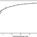
In summary, the series structure allows the classifiers to gather, with each step, context information from a progressively larger image neighborhood to the pixel being classified, as occurs with a convolutional ANN. The pixel values are sampled with a stencil neighborhood over each pixel, containing the pixels within the stencil (Fig. 10.5). The probability map feature vector is also obtained with a stencil neighborhood placed over each pixel containing information about the classes, as determined by the previous classifier. Indirectly, the classification from the previous ANN contains information about features in surrounding pixels, that is not represented in the original feature set. This allows the subsequent networks in the series (Fig. 10.6) to make decisions about the membrane classification utilizing nonlocal information. Put differently, each stage in the series accounts for larger structures in the data, taking advantage of results from all the previous networks. This results in membrane detection that improves after each network in the series. Figure 10.7 visually demonstrates the classification improving between ANNs in the series as gaps in weak membranes are closed and intracellular structures are removed with each iteration in the series. The receiver operating characteristic (ROC) curves in Fig. 10.8 also demonstrate the increase in detection accuracy after each ANN in the series. Notice that the results converge after a few stages.
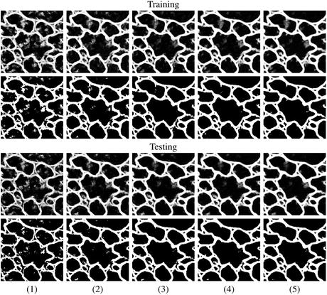
Fig. 10.7
Example output using the same image, first as part of a training set (top two rows), and then separately, as part of a testing set (bottom two rows), at each stage (1–5) of the network series. The output from each network is shown in rows 1 and 3. Rows 2 and 4 demonstrate the actual membrane detection when that output is thresholded. The network quickly learns which pixels belong to the membranes within the first 2–3 stages and then closes gaps in the last couple of stages
Fig. 10.8
ROC curves for the (a) training data and (b) testing data for each stage of the network on the C. elegans dataset
Combining the original image features with features sampled from the output of the previous classifier is important because, in this way, the membrane structure relevant for detection is enforced locally and then again at a higher level with each step in the series of classifiers. One of the advantages of this approach is that it provides better control of the training, allowing the network to learn in steps, refining the classification at each step as the context information it needs to correctly segment the image increases. Again, note that the membrane structure is learned directly from the data. Compared to a single large network with many hidden layers and nodes, such as the convolutional ANN of Jain et al. [39], the proposed classifier is easier to train. This is mainly because each of the ANNs has a relatively small number of parameters. For example, for a single ANN, the number of parameters needed is approximately 500 for the first ANN and 1,100 for the remaining ANNs in the series. The number of weights in an ANN with a single-hidden layer is given by  , where n is the number of inputs and h is the number of nodes in the hidden layer. For the first ANN in the series, n = s, where s is the number of points in the stencil. For the remaining ANNs in the series, n = 2s, since the original image and the output from the previous classifier are each sampled once. The total number of parameters across the whole series totals to approximately 5,000. In contrast, a convolutional ANN needs (n + 1)h for the first layer, and (n h + 1)h for the remaining layers, an h 2 dependence [39]. Hence, much less training data is needed in this approach, which is hard to obtain, since the ground truth must be hand labeled.1 Furthermore, the training is simpler since backpropagation is less likely to get stuck on local minima of the performance surface [89, 90], and the network will train much faster. Moreover, this accounts for a smaller and simpler network which can be trained from smaller numbers of features in the input vector. The series of ANNs is much more attractive to train, as opposed to using a single large network with many hidden layers and nodes. A single large network would be time consuming and difficult to train due to the many local minima in the performance surface.
, where n is the number of inputs and h is the number of nodes in the hidden layer. For the first ANN in the series, n = s, where s is the number of points in the stencil. For the remaining ANNs in the series, n = 2s, since the original image and the output from the previous classifier are each sampled once. The total number of parameters across the whole series totals to approximately 5,000. In contrast, a convolutional ANN needs (n + 1)h for the first layer, and (n h + 1)h for the remaining layers, an h 2 dependence [39]. Hence, much less training data is needed in this approach, which is hard to obtain, since the ground truth must be hand labeled.1 Furthermore, the training is simpler since backpropagation is less likely to get stuck on local minima of the performance surface [89, 90], and the network will train much faster. Moreover, this accounts for a smaller and simpler network which can be trained from smaller numbers of features in the input vector. The series of ANNs is much more attractive to train, as opposed to using a single large network with many hidden layers and nodes. A single large network would be time consuming and difficult to train due to the many local minima in the performance surface.Multi-scale Series of ANN Pixel Classifier
In this section, we discuss how more information can be obtained by using a scale-space representation of the context and allowing the classifier access to samples of context at different scales. It can be seen from (10.3) that context image provides prior information to solve the MAP problem. Although the Markov assumption is reasonable and makes the problem tractable, it still results in a significant loss of information from global context because it only uses local information obtained from the neighborhood area. However, it is not practical to sample every pixel in a very large neighborhood area of the context due to computational complexity problem and overfitting. The series classifiers exploit a sparse sampling approach to cover large context areas as shown in Fig. 10.5. However, single pixel contextual information in the finest scale conveys only partial information about its neighborhood pixels in a sparse sampling strategy while each pixel in the coarser scales contains more information about its neighborhood area due to the use of averaging filters. Furthermore, single pixel context can be noisy whereas context at coarser scales is more robust against noise due to the averaging effect. In other words, while it is reasonable to sample context at the finest level a few pixels away, sampling context at the finest scale tens to hundreds of pixels away is error prone and results in a non-optimal summary of its local area. We will show how more information can be obtained by creating a scale space representation of the context and allowing the classifier access to samples of small patches at each scale. Conceptually, sampling from the scale space representation increases the effective size of the neighborhood while keeping the number of samples small.
Multi-scale Contextual Model
The multi-scale contextual model is shown in Fig. 10.9. In the conventional series structure, the classifiers simply take sparsely sampled context together with input image as input. In the multi-scale contextual model, each context image is treated as an image and a scale-space representation of context image is created by applying a set of averaging filters. This results in a feature map with lower resolution that is robust against the small variations in the location of features as well as noise.Figure 10.10 shows the multi-scale sampling strategy versus the single-scale sampling strategy. In Fig. 10.10b the classifier can have as an input the center 3 ×3 patch at the original scale and a summary of eight surrounding 3 ×3 patches at a coarser scale (The green circles denote the summaries of dashed circles). The green circles in Fig. 10.10b are more informative and less noisy compared to their equivalent red circles in Fig. 10.10a
 Computational Intelligent Image Analysis for Assisting Radiation Oncologists’ Decision Making in Radiation Treatment Planning
 The Role of Content-Based Image Retrieval in Mammography CAD
 Liver Volumetry in MRI by Using Fast Marching Algorithm Coupled with 3D Geodesic Active Contour Segmentation
 Computational Anatomy in the Abdomen: Automated Multi-Organ and Tumor Analysis from Computed Tomography
 Subtraction Techniques for CT and DSA and Automated Detection of Lung Nodules in 3D CT
 Bone Suppression in Chest Radiographs by Means of Anatomically Specific Multiple Massive-Training ANNs Combined with Total Variation Minimization Smoothing and Consistency Processing


Related posts:
Computational Intelligent Image Analysis for Assisting Radiation Oncologists’ Decision Making in Radiation Treatment Planning
The Role of Content-Based Image Retrieval in Mammography CAD
Liver Volumetry in MRI by Using Fast Marching Algorithm Coupled with 3D Geodesic Active Contour Segmentation
Computational Anatomy in the Abdomen: Automated Multi-Organ and Tumor Analysis from Computed Tomography
Subtraction Techniques for CT and DSA and Automated Detection of Lung Nodules in 3D CT
Bone Suppression in Chest Radiographs by Means of Anatomically Specific Multiple Massive-Training ANNs Combined with Total Variation Minimization Smoothing and Consistency Processing
Stay updated, free articles. Join our Telegram channel
Full access? Get Clinical Tree
