Fig. 6.1
Overview of our computerized MR liver volumetry scheme
(6.1)
(6.2)
(6.3)
(6.4)
(6.5)
In the following step, the shape of the liver was estimated roughly by a fast marching algorithm [21, 22]. This algorithm was initially proposed as a fast numerical solution of the Eikonal equation:

where F is a speed function and T is an arrival time function. The algorithm requires five to eight initial seed points. From the initial location (T = 0), the algorithm propagates the information in one way from the smaller values of T to larger values based on the first order scheme. This algorithm consists of two main processes. First, all grid points generated from the entire region were categorized into three categories: seed points corresponding to the initial location were categorized into Known; the neighbors of Known points were categorized into Trial with the computed arrival time; and all other points were categorized into Far that the arrival time was set to infinity. An iterative process served points in the Trial and Far list. The Trial point p with the smallest T value was chosen and moved to the Known. The arrival time of neighbors of p was recomputed based on the first order scheme, and the Far points that are neighbors of p were moved to the Trial. This iterative process was terminated when the maximum number of iterations was reached. The salient point of this algorithm is to use a heap data structure that can locate points with the smallest T value rapidly. The output of the fast marching algorithm is a time-crossing map indicating the time traveling to each point. It forms a rough shape of the liver in MR images.
(6.6)
A 3D geodesic active contour algorithm [23] was employed to refine the initial surface determined by the time-crossing map in order to determine the liver boundaries more precisely. This algorithm is based on the relation between active contours and the computation of geodesic or minimal distance curves, which allows boundary detection with large variations of gradients, including gaps. Let ψ(p, t) be a level set function with the initial surface corresponding to ψ(p, t) = 0 (Fig. 6.2). This level set function is then evolved to fit the form of liver following the partial differential equation:
where A(∙) is an advection vector function, F(∙) is a propagation (or expansion) function, and Z(∙) is a spatial modifier function for the mean curvature κ. The scalar constants α, β, and γ allow trading off among three terms: advection, propagation, and curvature. The algorithm requires an initial zero level set containing an initial surface that roughly approximates the liver boundaries. The initial surface was propagated with speed and direction (outwards, inwards) controlled by the propagation function. The spatial modifier term controls the smoothness of the surface where regions of high curvature are smoothed out. The level set evolution was terminated when the convergence criterion or the maximum number of iterations was reached. The convergence criterion was defined in terms of the root mean squared (RMS) change in the level set function. The evolution was considered to be converged if the RMS change is below a predefined threshold. The liver regions extracted by the geodesic active contour algorithm were used to calculate the liver volume. The intermediate results of our scheme for an example case are illustrated in Fig. 6.3. The original MR image in Fig. 6.3a was passed into the anisotropic diffusion filter to reduce noise while preserving the major liver structures such as the portal vein and liver boundary, as shown in Fig. 6.3b. The noise-reduced image was then passed through a Gaussian gradient magnitude filter to enhance the boundaries, as shown in Fig. 6.3c. The edge potential image generated from the enhanced image using the sigmoid gray-scale converter was applied to the fast marching algorithm to generate the initial contour, as shown in Fig. 6.3d. The liver was extracted more precisely by using the geodesic active contour algorithm, as shown in Fig. 6.3e. Corresponding between computer-based liver segmentation (red contour) and “gold-standard” manual liver segmentation (blue contour) is shown in Fig. 6.3f. Liver volume was computed using the extracted regions.
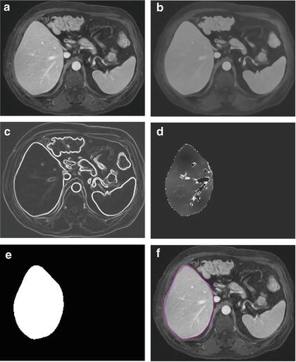
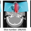
Fig. 6.2
Concept of level set method
(6.7)
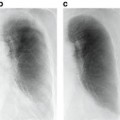
Fig. 6.3
Examples of the resulting images at each step in our automated volumetry scheme. (a) Original axial MR image of the liver. (b) 3D anisotropic diffusion noise reduction. (c) 3D gradient magnitude filter. (d) 3D fast marching algorithm. Time-crossing map indicates the traveling time to each voxel. The majority of vessels inside the liver are excluded at this stage. (e) 3D geodesic active contour segmentation. (f) Corresponding computer-based liver segmentation (red contour) and “gold-standard” manual liver segmentation (blue contour)
Evaluation Criteria
The liver volumes obtained by using our computerized scheme were compared to the “gold-standard” manual volumes determined by the radiologist. The definitions used in evaluation of a computerized liver segmentation compared to the gold-standard manual liver segmentation are shown in Fig. 6.4. True-positive (TP) segmentation was defined as an overlapping region (gray color) between the computerized liver segmentation (indicated by a red contour), C, and a gold-standard manual segmentation (indicated by a blue contour), G; i.e., TP = G ∩ C. False-positive (FP) segmentation (red region) was defined by FP = C − TP. False-negative (FN) segmentation (blue region) was defined by FN = G − TP. True-negative (TN) segmentation was defined by TN = I − G ∪ C, where I is the entire image. We define accuracy, specificity, and sensitivity of the segmentation as
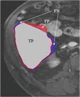
Fig. 6.4
Definitions of true-positive (TP) (gray region), false-positive (FP) (red region), and false-negative (FN) segmentation (blue region) in evaluation of computerized liver segmentation (red contour) compared to “gold-standard” manual segmentation (blue contour)
(6.8)
(6.9)
(6.10)
The Dice measurement representing the fraction of the overlapping volume and the volume of two segmentation methods is given by
(6.11)
We also determine the percentage volume error (E) for each computerized volume (V c) and the gold-standard manual volume (V m) as
(6.12)
The association between the computerized volumetry and the manual volumetry was measured by the Pearson product–moment correlation coefficient (r). The significance of correlation coefficient was evaluated by using the Student t test. An agreement between two measurements was assessed by using the intraclass correlation coefficient (ICC) [24, 25]. The two-way random single measure model, ICC(2,1), was used because we assumed that the cases were chosen randomly from population and each case was measured by two volumetric methods. The ICC(2,1) was defined by the following equation:
where n is the number of cases, k is the number of raters (i.e., volumetric methods), BMS is the between-cases mean square, EMS is the error mean square, and RMS
 Computational Intelligent Image Analysis for Assisting Radiation Oncologists’ Decision Making in Radiation Treatment Planning
 The Role of Content-Based Image Retrieval in Mammography CAD
 Brain Disease Classification and Progression Using Machine Learning Techniques
 Subtraction Techniques for CT and DSA and Automated Detection of Lung Nodules in 3D CT
 Bone Suppression in Chest Radiographs by Means of Anatomically Specific Multiple Massive-Training ANNs Combined with Total Variation Minimization Smoothing and Consistency Processing
 Image Segmentation for Connectomics Using Machine Learning


(6.13)
Related posts:
Computational Intelligent Image Analysis for Assisting Radiation Oncologists’ Decision Making in Radiation Treatment Planning
The Role of Content-Based Image Retrieval in Mammography CAD
Brain Disease Classification and Progression Using Machine Learning Techniques
Subtraction Techniques for CT and DSA and Automated Detection of Lung Nodules in 3D CT
Bone Suppression in Chest Radiographs by Means of Anatomically Specific Multiple Massive-Training ANNs Combined with Total Variation Minimization Smoothing and Consistency Processing
Image Segmentation for Connectomics Using Machine Learning
Stay updated, free articles. Join our Telegram channel
Full access? Get Clinical Tree
