Fig. 1
Typical ultrasound images of (a) benign tumors (b) malignant tumors
Methods
Our proposed system for ovarian tumor classification is presented in Fig. 2. It consists of an online classification system (shown on the right side of Fig. 2) which processes a test image. This online system predicts the class label (benign or malignant) of the test image based on the transformation of the online gray scale feature vector by the training parameters determined by an off-line learning system (shown on the left side of Fig. 1). The off-line classification system is composed of a classification phase which produces the training parameters using the combination of gray scale off-line training features and the respective off-line ground truth training class labels (0/1 for benign/malignant). The gray scale features for online or off-line training are the same: Hu’s invariant moments, Gabor wavelet transform parameters, and entropies. Significant features among the extracted ones are selected using the t-test. We evaluated the probabilistic neural network (PNN) classifier. The best model parameter (σ) for which the PNN classifier performs the best is identified using genetic algorithm. The classifier robustness is evaluated using tenfold cross-validation. The predicted class labels of the test images and the corresponding ground truth labels (0/1) are compared to determine the performance measures of the system such as sensitivity, specificity, accuracy, and PPV.
Fig. 2
The proposed system for the ovarian tumor classification
In the remainder of this section, we describe the features, Gabor wavelet transform and entropy features, the PNN classifier, and the feature selection test (t-test) used in this work.
Feature Extraction
In this work, we have extracted seven Hu’s invariant moments, mean and standard deviation values of coefficients of Gabor wavelet transform at different angles and slices, and Yager and Kapur entropies. These features are briefly explained in this section.
Hu’s Invariant Moments
Moments and the related invariants have been extensively analyzed to characterize the patterns in images in a variety of applications. 2D moment of an image f (x, y) is defined by
(1)
For p, q = 0, 1, 2…, the central moment is defined as
where  and
and  are the centroid of the image. Here, we consider binary image. In a binary image, m 00 is the area of the image. The normalized central moment of order (p + q) is defined as

(2)
and are the centroid of the image. Here, we consider binary image. In a binary image, m 00 is the area of the image. The normalized central moment of order (p + q) is defined as(3)
For p, q = 0, 1, 2, 3 …, where  . From this normalized central moment Hu [31] defined seven values through order three that are invariant to object scale, position, and orientation. These seven moments are defined as:
![$$ \begin{array}{c}{M}_5=\left({\eta}_{30}-3{\eta}_{12}\right)\left({\eta}_{30}+{\eta}_{12}\right)\Big[({\eta}_{30}+{\eta}_{12}){}^2\\ {}\kern1.12em -3{\left({\eta}_{21}-{\eta}_{03}\right)}^2\left]+\right(3{\eta}_{21}-{\eta}_{03}\left)\right({\eta}_{21}+{\eta}_{03}\Big)\\ {}\kern1.12em \left[3{\left({\eta}_{30}+{\eta}_{12}\right)}^2-\right({\eta}_{21}+{\eta}_{03}\left){}^2\right]\end{array} $$](/wp-content/uploads/2016/09/A301939_1_En_27_Chapter_Equ8.gif)
![$$ \begin{array}{c}{M}_6=\left({\eta}_{20}-{\eta}_{02}\right)\;\left[\right({\eta}_{30}+{\eta}_{12}\left){}^2-\right({\eta}_{21}+{\eta}_{03}\left){}^2\right]\\ {}\kern1em +4{\eta}_{11}\left({\eta}_{30}+{\eta}_{12}\right)\left({\eta}_{21}+{\eta}_{03}\right)\;\end{array} $$](/wp-content/uploads/2016/09/A301939_1_En_27_Chapter_Equ9.gif)
![$$ \begin{array}{c}{M}_7=\left(3{\eta}_{21}-{\eta}_{03}\right)\left({\eta}_{30}+{\eta}_{12}\right)\\ {}\kern1em \left[{\left({\eta}_{30}+{\eta}_{12}\right)}^2-3({\eta}_{21}+{\eta}_{03}){}^2\right]\\ {}\kern1em +\left(3{\eta}_{12}-{\eta}_{30}\right)\left({\eta}_{21}+{\eta}_{03}\right)\\ {}\kern1em \left[3{\left({\eta}_{30}+{\eta}_{12}\right)}^2-({\eta}_{21}+{\eta}_{03}){}^2\right]\end{array} $$](/wp-content/uploads/2016/09/A301939_1_En_27_Chapter_Equ10.gif)
. From this normalized central moment Hu [31] defined seven values through order three that are invariant to object scale, position, and orientation. These seven moments are defined as:(4)
(5)
(6)
(7)
(8)
(9)
(10)
Gabor Wavelet Transform
Among various wavelet bases, Gabor function provides the optimal resolution in both the time (spatial) and frequency domains. It has both multi-resolution and multi-orientation properties and can effectively capture the local spatial frequencies [32]. Two-dimensional Gabor function [33] is a Gaussian modulated complex sinusoid and can be written as
(11)
Here, ω is frequency of the sinusoid and σ m and σ n are the standard deviations of the Gaussian envelopes. 2D Gabor wavelets are obtained by dilation and rotation of the mother Gabor wavelet ψ(m,n) using
![$$ \begin{array}{l}{\psi}_{i,k}\left(m,n\right)={a}^{-l}\psi \left[{a}^{-l}\right( mcos\theta + nsin\theta \Big),\\ {}\kern5em {a}^{-l}\left(- msin\theta + ncos\theta \right)\Big],a>1\end{array} $$
” src=”/wp-content/uploads/2016/09/A301939_1_En_27_Chapter_Equ12.gif”></DIV></DIV><br />
<DIV class=EquationNumber>(12)</DIV></DIV>where <SPAN class=EmphasisTypeItalic>a</SPAN> <SUP>− <SPAN class=EmphasisTypeItalic>l</SPAN> </SUP>is a scale factor, <SPAN class=EmphasisTypeItalic>l</SPAN> and <SPAN class=EmphasisTypeItalic>k</SPAN> are integers, the orientation <SPAN class=EmphasisTypeItalic>θ</SPAN> is given by <SPAN class=EmphasisTypeItalic>θ</SPAN> = <SPAN class=EmphasisTypeItalic>kπ</SPAN>/<SPAN class=EmphasisTypeItalic>K</SPAN>, and <SPAN class=EmphasisTypeItalic>K</SPAN> is the number of orientations. The parameters <SPAN class=EmphasisTypeItalic>σ</SPAN> <SUB><SPAN class=EmphasisTypeItalic>m</SPAN> </SUB>and <SPAN class=EmphasisTypeItalic>σ</SPAN> <SUB><SPAN class=EmphasisTypeItalic>n</SPAN> </SUB>are calculated according to the design strategy proposed by Manjunath et al. [<CITE><A href=]() 33]. Given an image I(m,n), its Gabor wavelet transform is obtained as
33]. Given an image I(m,n), its Gabor wavelet transform is obtained as
where ∗ denotes the convolution operator. The parameters K and S denote the number of orientations and number of scales, respectively. The mean and the standard deviation of the coefficients are used as features and given by
(13)
(14)
The feature vector is then constructed using mean (μ l,k ) and standard deviation (std) (σ l,k ) as feature components, for K = 6 orientations and S = 4 scales, resulting in a feature vector of length 48, given by
(15)
In this work, we extracted 2D Gabor wavelet features at 0º, 30º, 60º, 90º, 120º, and 150º.
Entropy
Entropy is widely used to measure of uncertainty associated with the system. In this work, we have used Yager’s measure and Kapur’s entropy to estimate the subtle variation in the pixel intensities. Let f (x,y) be the image with N i (i = 0, 1, 2, 3, 4………….. L − 1) distinct gray levels. The normalized histogram for a particular region of interest of size (M × N) is given by
(16)
In this experiment, we considered α = 0.5 and β = 0.7
Feature Selection
Student’s t-test [35] is used to assess whether the means of a feature in two groups are statistically different from each other. The result of this test is the p-value. Lower p-value indicates that the two groups are well separated. Typically, features with p-values less than 0.05 are regarded as clinically significant.
Classification
The probabilistic neural network (PNN) model [36–38] is based on Parzen’s results on probability density function estimators [37]. PNN is a three-layer feed forward network consisting of an input layer, a pattern layer, and a summation layer. A radial basis function and a Gaussian activation function can be used for the pattern nodes. In this work, PNN model was implemented using radial basis function (RBF) mentioned below.
![$$ Q=f(x)= exp\left[-\frac{\left|\right|w-p\left|\right|{}^2}{2{\sigma}^2}\right] $$](/wp-content/uploads/2016/09/A301939_1_En_27_Chapter_Equ19.gif)
where σ is an smoothing parameter.
(19)
The net input to the radial basis transfer function is the vector distance between its weight vector w and the input vector p, multiplied by the bias b. The RBF has a maximum of 1 when its input is 0. As the distance between w and p decreases, the output increases. Thus, a radial basis neuron acts as a detector, which produces 1 whenever the input p is identical to its weight vector.
PNN is a variant of radial basis network. When an input is presented, the first layer computes distances d from the input vector to the training input vectors and produces a vector whose element indicates how close the input is to a training input. The second layer sums these contributions for each class of inputs to produce probabilities as its net output vector. Finally, a compete transfer function on the output of the second layer picks the maximum of these probabilities and produces a 1 for that class and a 0 for the other classes [37].
PNN Smoothing Parameter Tuning
The smoothing parameter (σ) which controls the scale factor of the exponential activation function should be chosen appropriately to get the highest accuracy of classification. The decision boundary of the classifier varies continuously from a nonlinear hyperplane when σ → 1 and when σ → 0 represents the nearest neighbor classifier. For each value of σ, there will be a value for accuracy. The classifier provides highest accuracy only for a particular σ depending on data characteristics [36]. The value of σ has to be evaluated experimentally. One solution is to use brute force technique which requires lot of runs each for the possible σ. Another solution is to define the overall accuracy of the classifier for an initial σ as the fitness function in an evolutionary algorithm and the algorithm can be iterated over generations with a fixed population. In this work, we have used genetic algorithm (GA) [39, 40] which uses principles from natural genetics.
Genetic Algorithm (GA)
Genetic algorithm [37, 39, 40] is a global optimization strategy used in this experiment to tune the smoothing parameter of PNN and to obtain the highest possible accuracy. GA operates in binary-coded string space rather than in the original real feature space. Therefore, the features and its solution are to be encoded into binary strings which are called chromosomes, and finally they are decoded into the real numbers. The algorithm consists of three basic operations, reproduction, crossover, and mutation. A given population size is defined; in our experiment we have assumed population size of 20. Initially, 20 different random σs are assumed and the corresponding average accuracy over 10-folds is computed. The fitness function is made equal to the reciprocal of average accuracy over 10-folds. The problem is to maximize the average accuracy which reflects into minimization of the fitness function. In the 20 initial instances with different σs, the fittest solutions with higher fitness value are selected and reproduced in the next generation. A given crossover probability is defined (in our case we chose 0.8), and the proportion of population are chosen (in our case it will be 80 % of population size of 20 which is equal to 16). Randomly a given crossover site is taken and the chromosome (or bit string) is broken into two parts for each population. Two such strings belonging to different populations are joined at crossover site and new population is obtained. Also a given mutation probability is defined (in our case it is 0.05). Generally it is kept very low in comparison with natural genetics, and the corresponding proportion of bits of binary string is flipped. The three operations are continued in every generation. If there is no change in fitness function over iterations, the algorithm is terminated and the corresponding best fitness is the solution of the problem.
Results
Selected Features
Table 1 shows the mean ± standard deviation values of the various significant features for the benign and malignant classes. Since the p-value is less than 0.05, these features can be used to discriminate the two classes with higher accuracy. It can be seen from our results that the mean value of Gabor wavelet coefficients and Hu’s invariant moments are higher for malignant images than the benign images. This may be because the malignant images have a relatively complex texture marked by increased randomness in the intensity distributions which lead to higher mean Gabor and Hu’s invariant moment values.
Table 1
Mean ± standard deviation values of the various features for the benign and malignant classes
Features | Benign | Malignant | p-value |
|---|---|---|---|
Entropy | |||
Yager | 0.9962 ± 0.0002 | 0.9961 ± 0.0001 | <0.0001 |
Kapur | 7.829 ± 0.1747
Related posts:Stay updated, free articles. Join our Telegram channel
Full access? Get Clinical Tree
 Get Clinical Tree app for offline access

| ||