Applications of Hyperpolarized Agents in Solutions

Mouse (rapid bolus i.v.)

Rat (rapid bolus i.v.)

Dog (rapid bolus i.v.)

Max vol. (mL/kg)

Max rate (mL/s)

Max vol.

(mL/kg)

Max rate (mL/s)

Max vol. (mL/kg)

Max. rate

Ref. (9)

0.05

2.5

Dose given over 1 min

The physiological effect of a rapid bolus on heart and lung is buffered when it is administered in a peripheral vein or artery. The bolus is in this way more effectively diluted in blood and the peak concentration reaching key organs is reduced. For central venous administrations, it is strongly encouraged to confirm that the procedure is tolerated by administration of saline/osmotic control, before the study with the hyperpolarized agent is initiated.

For experiments of longer duration (>60 min) and experiments including surgical procedures, do ensure that the fluid balance of the animal is maintained according to standard practices.

1.1 Pulse Sequences for Angiography and Perfusion

In angiography and perfusion studies the imaging strategy is reduced to the visualization (spatial encoding) of the MR-active nuclei. The hyperpolarized agent should preferably not be metabolically active. First, this will facilitate quantitative analysis. Secondly, it means that the applied pulse sequence does not need to resolve the multiple resonance frequencies of the injected molecule and any metabolites. Indeed, it may even be desirable to suppress metabolite signals for vascular applications. Consequently, the requirements of a MR pulse sequence for these applications “vascular hyperpolarized imaging,” are very similar to clinical routine angiographic or perfusion imaging, except for the differences imposed by the non-equilibrium magnetization. The intra-voxel spin dephasing caused by flow and acceleration needs to be suppressed and the sequence needs to be able to deal with inflow/outflow effects.

Most hyperpolarized MR vascular studies have been based on variations of fully balanced steady-state free precession (bSSFP) pulse sequences (11–14). The general outline of this sequence is shown in Fig. 1. When this sequence is used for conventional MR imaging, the flip angle is in the range 10–60° and a number of TR periods and pre-pulses are applied to establish steady state before starting the data collection, ensuring stable signal amplitude during the readout (15–17). In hyperpolarized imaging, the polarization (and thus the signal) irreversibly decays toward thermal equilibrium, which is essentially zero, and a steady state is never established (13). Instead, the collection of data takes place during a transient phase. In this situation, with an α/2 pre-pulse (18) the optimal flip angle, α, is found to be 180° (19) resulting in a sequence that is similar to fast spin echo (FSE) (20) sequences.

Fig. 1.

The bSSFP sequence. In order to generate an n × m image matrix the signal during each sampling interval is sampled n times and the total number of echoes is m. The box indicated using dashed line shows the part of the sequence that is being repeated.

The bSSFP sequence takes advantage of the long T ₂-relaxation time of the hyperpolarized ¹³C spins. Furthermore, the rewinding of the gradients in all directions during each TR interval minimizes loss of signal due to moving spins. The sequence is based on a single excitation; the 90° pre-pulse flips all spins within the imaged slice into the transverse plane and the following 180° pulses generate a series of spin echoes. By applying a centric phase-encoding scheme, the effect of signal amplitude decay due to imperfect refocusing pulses and finite T ₂ relaxation is minimized. The signal is sampled as a full spin echo with its maximum in the center of the TR interval. This ensures that all effects from J-couplings are suppressed as in the case when the imaging agent hydroxyethyl-[1-¹³C]propionate, generated through the PHIP (para-hydrogen induced polarization, cf. Chapter 11) method, is used.

It should be noted that the low gyromagnetic ratio of ¹³C is a liming factor when reducing TE and TR times, as the gradient integral required to achieve a given field of view scales with γ ⁻¹. However, implementation of bSSFP sequences on clinical MR scanners and the use of state-of-the-art gradient systems have been demonstrated successfully, and scan times of the order of 300 ms (1) with a matrix size of 128 × 64 (TR/TE of 6.6/3.3 ms) have been achieved.

1.2 Pulse Sequences Adapted for Metabolic Imaging and pH Mapping

A pulse sequence for metabolic imaging needs to be capable of resolving the resonance frequencies of the injected molecule as well as molecules generated by the metabolic processes. Therefore, in addition to the previous section, the spectral dimension has to be considered. The simplest approach is to apply a modified 2D or 3D chemical shift imaging (CSI) FID pulse sequence. These types of sequences require a number of excitation pulses that are equal to the number of voxels in the final raw data matrix (disregarding zero filling). Phase-encoding gradients are applied in two or three directions prior to the signal acquisition, which renders this sequence time consuming. However, the sequence is easy to adapt and consequently it has been used in most metabolic imaging with hyperpolarized molecules. It has also been used to demonstrate in vivo pH measurements (21). The sequence is outlined in Fig. 2a together with its k-space sampling scheme in Fig. 2b.

Fig. 2.

The CSI pulse sequence. The left-hand side (a) outlines the sequence and the right-hand side (b) shows the corresponding k-space sampling scheme. In order to get an n × m image matrix the sequence is repeated n × m times. Both x and y gradients are used to phase encode the signal. The x gradient is changed n times and the y gradient m times. The FID signal is sampled for each repetition and the readout time determines the chemical shift frequency resolution. The position of the sampling window is indicated in (a) and its corresponding position in the k-space is indicated in (b). Note that during one repetition only data along one of the k-space track is collected.

When proton CSI is performed the TR of the sequence may typically be several seconds. However, in the case of hyperpolarized CSI, the objective is to minimize TR, typically to less then 100 ms. The length of the sampling window is chosen to assure that the peaks from the injected substance and molecules created by metabolic processes are resolved and the tail of the FID may be truncated. This means that only a small part of the FID is sampled and the truncation introduces a line broadening. The flip angle of the excitation pulses are selected to match the total number of repetitions. Each sampling interval is followed by spoiler gradients in order to suppress the signal from magnetization remaining in the transverse plane. A sampling of the FID signal is used, and not a spin echo, as the application of a 180° pulse would alter the phase of not only the excited spins but also the spins still in the longitudinal direction.

In the k-space diagram in Fig. 2, only two dimensions are shown: the k _x-axis, which after the reconstruction will form the spatial x-dimension, and the k _f-axis, the evolution in the time dimension which after the reconstruction will form the frequency dimension (the chemical shift dimension). From the k-space diagram it follows that the center is not collected during this type of sequence and also that the spatial dimensions are sampled more coarsely than the time dimension, which results in low resolution spatial images.

In summary, the high resolution of the CSI sequence in the spectral domain makes it useful in situations where complicated spectra with several peaks are evaluated. The sequence puts emphasis on collecting spectral information with coarse localization, since the time window for sampling the signal is limited by the T ₁ of the hyperpolarized nuclei and the dynamics of metabolism. A way of reducing the scan time is to not sample the corners of k-space. However, even a relatively low spatial resolution matrix of 16 × 16 will result in a total scan time of around 12 s (22).

In order to overcome the obvious inefficiencies of the basic CSI FID sequence in the context of hyperpolarized MR imaging, different multi-echo concepts have been developed (23). The CSI FID sequence may be extended to a multi-gradient echo sequence by adding alternating readout gradients. In the most extreme case, a large number of gradient echoes will result in a trajectory that covers a k-space volume sufficient to be reconstructed into a 3D/4D matrix with two/three spatial dimensions and one frequency dimension. The alternating gradient approach is similar to the way that the readout is performed in an echo planar imaging sequence. Consequently, when this is applied to a long echo train, in order to allow for spectroscopic information to be resolved and collected, the acronym EPSI, echo planar spectroscopic imaging, is used to describe this sequence (24). The total length of the echo train is only limited by the ${\textrm{T}}_2^*$ of the imaged nucleus. In order to account for finite ${\textrm{T}}_2^*$ , EPSI may be implemented as a multi-shot technique where a low flip angle excitation pulse is used and the sequence is repeated in order to obtain the desired spatial as well as spectroscopic resolution.

The echo train readout may be performed using the flyback technique (25) allowing for a read out k-space trajectory that is less sensitive to error in timing relative to the traditional alternating gradient readout used in most EPI implementations. This sequence has been applied for 2D and 3D hyperpolarized imaging (26). The data acquisition part of the sequence is outlined in Fig. 3a together with its k-trajectory in Fig. 3b. During the reconstruction, the tilted sample points are interpolated onto a rectilinear grid by the use of a sinc interpolation (27, 28). The equivalent of a sinc interpolation in the time dimension is a phase shift in the spectral dimension (29). Consequently, this interpolation may be performed by applying a 1D Fourier transform along the time dimension (the k _f-direction in Fig. 3b). The phase shift procedure is then carried out on a sample point-to-sample point basis using (25):

$p{'_{{\textrm{sn}}}} = {p_{{\textrm{sn}}}}{{\textrm{e}}^{\left[ {\frac{{{\textrm{i2}}\pi sn\Delta t{B_{\textrm{s}}}}}{S}} \right]}}$

([1])

where p _sn is the nth sample within the spatial k-space sample s (the gradient echo no s), Δt is the distance between spatial k-space samples along the k _f-dimension, B _s is the spectral bandwidth, defined as the inverse of the time between the start of two consecutive sample intervals, and S is the total number of sampling intervals.

Fig. 3.

The EPSI pulse sequence with a flyback gradient scheme. The left-hand side (a) outlines the sequence and the right-hand side (b) shows the corresponding k-space sampling scheme. In order to acquire a data matrix with the spatial dimensions n × m and f points in the frequency dimension, the readout scheme is repeated m times. During each repetition the phase-encoding gradient, y, applied before the readout is changed. The series of gradient echoes are then sampled during the intervals S1, S2,…, Sf. During each sampling window the signal is sampled n times. The corresponding k-space positions of the sampling windows (S1,…, Sf) during each repetition are indicated in (b).

The EPI method has also been combined with spectral–spatial RF pulses in order to suppress the signal emanating from the outside of the volume of interest (30), multiband excitations in order to excite the metabolites with different effective flip angles (31), and ¹H decoupling techniques (32). A further extension of the k-space sampling is to replace the rapidly alternating readout gradient with a gradient scheme that will form a spiral trajectory in k-space (33, 34). This method has been applied to hyperpolarized imaging (35) and a temporal resolution of around 1 s has been demonstrated (36).

The EPSI sequence utilizes the available magnetization in a much more efficient way than the traditional CSI sequence with respect to spatial resolution. It also makes it possible to collect a 4D dataset (three spatial dimensions and one time dimension) (37) but it is still mainly a spectroscopic sequence and not an imaging sequence. In order to create metabolite maps, it depends on the resolution in the time/frequency dimension to separate information/signal from the injected substance and its metabolites.

When the spectrum is sparse and chemical shifts of the injected substance and its metabolites are known, a more efficient pulse sequence and post-processing procedure can be designed, which drastically reduces resolution in the spectral domain. This overcomes the trade-off between spatial and spectral sampling requirements by leaving more time for the spatial encoding. This idea has been applied in the case of hyperpolarized [1-¹³C]pyruvate to create a multi-echo bSSFP pulse sequence (38). The basic outline of this sequence is shown in Fig. 4a together with a part of its k-space trajectory in Fig. 4b.

Fig. 4.

The multi-echo bSSFP sequence used to generate maps of hyperpolarized [1-¹³C]pyruvate and its metabolites. The left-hand side (a) outlines the sequence and the right-hand side (b) shows the corresponding k-space sampling scheme. In order to generate maps with the matrix dimension n × m, the number of samples per echo is n and the number of phase-encoding interval is m. The number of echoes, S1, …, S5, within a phase-encoding interval determines the number of resonance peaks that will be possible to resolve. The corresponding k-space positions of the sampling windows (S1, …, Sf) during one repetition are indicated in (b). In this example, four metabolite maps may be calculated together with a B0 map.

The main feature of this class of pulse sequences is that it acquires images with high resolution in the spatial domain. The gradient schema mimics the one used in the GREASE sequence (39) but the phase encoding is performed once in the beginning and rewound at the end of each interval between the 180° refocusing pulses. This results in the same phase encoding for all generated echoes. The generated echoes will be a superposition of the signals from all metabolites in the imaged volume. At the position of the central echo, which is a true spin echo, the signals from all metabolites will be in phase and this echo is also compensated for main field inhomogeneities. The k-space trajectory is designed to allow for separation of the signals arising from the different metabolites during post-processing. This requires prior knowledge of the phases of all the metabolites at the time of all echoes. The separation of the individual echoes is contingent on the specific chemical shift separation of the signals. As such, the suggested sampling scheme has many similarities with the Dixon technique (40, 41) suggested for separating water and fat in clinical proton imaging. An extension of the classical Dixon method has been suggested by Reeder et al. (42). In this approach, the minimum number of echoes required to reconstruct a certain number of MR signals equals the number of peaks that need to be resolved plus one. Furthermore, the reconstruction method is able to correct for phase errors caused by inhomogeneities in the main magnetic field. Alternatively, rather than making the B ₀ map an output of the reconstruction, prior knowledge about the spatial variation of B ₀ (from a ¹H MR field map of the same field of view) could be used to constrain the reconstruction. Different methods have been demonstrated for reconstructing the metabolic maps and detailed description may be found elsewhere (38, 43). Implementations of the multi-echo bSSFP pulse sequence combined with an interactive post-processing make it possible to reduce the scan time dramatically (38). In Fig. 5, a set of images generated using this approach is shown. The sequence was executed 25 s after an i.v. injection of hyperpolarized ¹³C-pyruvate into a full size pig. The total scan time was 520 ms making it possible to collect all data within one heartbeat.

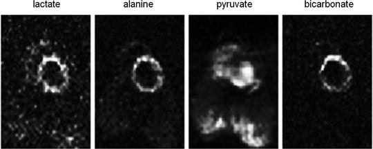
Fig. 5.

Generated metabolite maps after the injection of hyperpolarized [1-¹³C]pyruvate and using a multi-echo bSSFP sequence The matrix size is 64 × 32 and the images demonstrate a slice through the left ventricle of the pig. The lactate, alanine, and bicarbonate are all metabolites after the injected pyruvate. The total scan time was 520 ms.

1.3 Summary

In this section, MR pulse sequences for hyperpolarized MR have been reviewed briefly. The main aspects to be aware of are as follows:

Hyperpolarized MR is limited by the relaxation times of the non-equilibrium magnetization.
Long T ₂ times of hyperpolarized ¹³C-labeled molecules in solutions allow for multi-echo sampling schemes.
In applications such as metabolic imaging or pH mapping, a further trade-off is encountered due to the necessity to also sample the spectral domain.
This trade-off can be partially overcome if prior knowledge about the chemical shifts of the MR signals of interest allows for sparse spectral sampling, thus retaining the spatial resolution of conventional MR imaging.

2 Angiography, Perfusion, and Interventional Procedures

In conventional vascular proton imaging, the contrast medium, CM, decreases the protons relaxation times in the vicinity of the paramagnetic center of the injected molecules. Depending on the applied pulse sequence, the passage of a CM bolus will result in an increase or a decrease of the MR signal and hence affect the contrast of the resulting MR image. However, the MR signal itself does not arise from the CM but the protons in the tissue. This is different compared to vascular imaging using hyperpolarized agents where the MR signal arises from the MR-active nuclei of the injected agent, e.g., ¹³C. Due to the low concentration of ¹³C in the body there is no background signal at all from tissues in the imaging volume.

In order to assure a strong signal in the image volume, a hyperpolarized agent for angiographic and perfusion imaging should preferably not be metabolically active. It should behave pharmacokinetically as an extra cellular fluid (ECF) MR contrast agent and mainly remain within the vascular bed at least during the first few re-circulations in the body. This requirement is fulfilled by hydroxyethyl-[1-¹³C]propionate which may be polarized using the PHIP method. Consequently, the majority of vascular imaging results presented in the literature have been generated using this model substance. It is not intended for human clinical use but its toxicity profile allows it to be used for preclinical animal model work.

The results described in the following section are obtained with this molecule unless otherwise indicated. The molecular weight of this substance is ∼130 g/mol and the in vivo ¹³C T ₁ and T ₂ of the substance have been determined to 45 and 6 s, respectively (2). The preparation for a hyperpolarized angiography or perfusion imaging experiment performed in a pig model may include the following steps (2):

The animal is premedicated with 10 mL ketamine (50 mg/mL Ketalar^®, Pfizer) intramuscularly and then the anesthesia is induced 20 min later with 10–15 mL thiopental sodium (25 mg/mL Pentothal natrium^®; Abbott) intravenously.
The pig is intubated and connected to a volume-controlled respirator delivering a gas mixture of 70% N₂O and 30% O₂. Normocapnia is maintained with tidal volumes of 12–14 mL/kg at a respiratory rate of 20 breaths per minute.
The anesthesia is maintained by intravenous infusion of a mixture (0.6–0.8 mL/min) of 10 mL midazolam (5 mg/mL Dormicum^®; Pharma Hameln Gmbh) + 40 mL ketamine + 20 mL Vecuron (2 mg/mL Norcuron^®; Organon) + 25 mL NaCl (9 mg/mL Fresenius Kabi).
During the session, the respiratory status is monitored by measuring blood gases (pO₂ and pCO₂) and pH. Rectal temperature is monitored and kept close to 38°C by a warming lamp and a heating pad.
Intravenous infusion is continuously given with Ringer acetate (Ringer-acetate^®, Fresenius Kabi) 3 mL/min.
In experiments involving catheterization, heparin 5000 IU (Heparin^®, Lovens Kemiske Fabrik) is given for a time interval of 3 min before the start procedure.
To confirm the position of catheters, one may inject 3 mL of iohexol 350 mg I/mL (Omnipaque^®; Amersham Health AS) to obtain X-ray angiograms.

2.1 Angiography

The first angiographic images following an i.v. injection of a hyperpolarized substance in a rat were presented by Golman et al. (44, 45). This was followed by the first dynamic angiography also performed in a rat model by Svensson et al. (19). The small animal model allowed the imaging to be performed in a preclinical animal MR scanner where large gradient amplitude combined with high slew rate made it possible to suppress flow artifacts and to generate images with high in-plane resolution. Although the PHIP method has been used in generating hyperpolarized agents for many vascular applications, the first angiogram obtained using the endogenous substance [¹³C]urea, was demonstrated using DNP (dynamic nuclear polarization, cf. chapter 11 of this book) as a polarization method (46).

Dynamic time series obtained during intra-arterial injection in pig models has demonstrated the possibilities for coronary angiography (1). Figure 7 shows images extracted from a dynamic acquisition, similar to the one described in (1), during which retrospective gating was applied. The images in Fig. 6 show flow artifacts due to the high velocity when the injected substance leaves the tip of the catheter. The time series were generated using the bSSFP pulse sequence implemented on a clinical MRI scanner capable of 40 mT m⁻¹ gradient amplitude. With maximum gradient amplitude and slew rate it was not possible to reach short enough TE to suppress the artifacts caused by moving ¹³C spins.

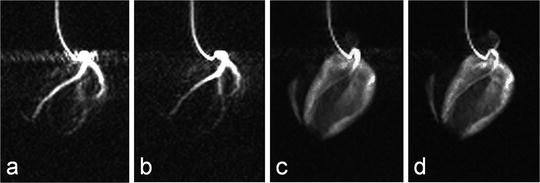
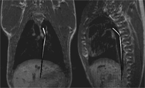
Fig. 6.

Images obtained during an intra-arterial injection through a catheter placed in the left coronary arteries. Images (a) and (b) are from the early phase of the injection, while images (c) and (d) are obtained after the injection has ended and the hyperpolarized molecule has reached the myocardium.

Fig. 7.

Two orthogonal ¹³C catheter-tracking images superimposed on proton road map images. The catheter was positioned inside the aorta.

2.2 Catheter Tracking

The possibility of visualizing a catheter in vivo, which contains flowing hyperpolarized ¹³C signal agent, has been demonstrated by Magnusson et al. (47). In this pilot study, a commercial three-lumen catheter was modified in order for two of the lumens to form a loop where the hyperpolarized ¹³C agent could flow without leaving the catheter. The third lumen was left open to enable injection of contrast agent into the endovascular space. Projection images of the catheter moving through the pig aorta to the renal arteries and to the aortic arch were acquired using a bSSFP pulse sequence. Two orthogonal projection images of the moving ¹³C-filled catheter were acquired with a temporal resolution of 658 ms. In Fig. 7, two orthogonal ¹³C images are shown. The catheter projections have been superimposed on proton road map images.

Once the catheter is in the desired position, a bolus of hyperpolarized solution can be injected through the third lumen. In this way, the catheter-tracking technique may be combined with the previously described intra-arterial injection methods. It may also serve as a basis for obtaining a series of dynamic images to allow for perfusion mapping (1, 3).

2.3 Perfusion

Clinical proton MR imaging has been extended to allow for the extraction of perfusion information. Typically, this is accomplished by observing the signal change during the passage of a paramagnetic contrast media bolus. A series of images covering the volume of interest is collected. Retrospectively, software is used to calculate relevant perfusion parameters such as the tissue blood flow, F, the tissue blood volume, V _b, and the mean transit time, MTT (48, 49). A similar approach has been suggested for hyperpolarized imaging agents (50). However, when a series of images are collected during the passage of a bolus containing hyperpolarized spins, the signal will depend on the applied RF pulses, the inflow and outflow of spins, and the irreversible relaxation. The spin polarization decreases irreversibly due to T ₁ relaxation. Therefore, the signal intensities as measured in a series of images will not directly be proportional to the concentration of the injected molecule. Consequently, it is not possible to correct for depolarization in the same manner in which decay is accounted for in imaging techniques based on radioactive tracers.

If the magnetization of the hyperpolarized compound is regarded as the tracer element, the concentration in a tissue voxel, C _T(t), at a time, t, can, according to Johansson (51), be related via a convolution integral to the concentration in a supplying artery, C _A(τ), that has entered the volume during the infinitesimally short interval dτ at time τ:

${C_{\textrm{T}}}(t) = F\int\limits_0^t {{C_{\textrm{A}}}(\tau ){R_M}(t - \tau ){\textrm{d}}\tau }$

([2])

where R _M(t−τ) is the residue function (52). It is defined as the fraction of tracer elements that entered the tissue volume at time t = τ, and still remains in the tissue volume at time t − τ. C _A(t) is often referred to as the arterial input function (AIF). The residue function needs to include a polarization function P that takes into account both T ₁ relaxation as well as polarization losses due to RF pulses. A detailed description of how to incorporate the effects of the depolarization during the image acquisitions and the influence of RF pulses in the case of perfusion assessment using a hyperpolarized tracer may be found in (51). If the concentration of the tracer in the tissue and in the arterial volume is known, the function F · R _M (t) may be determined by deconvolution and the tissue blood flow may be obtained. However, it should be noted that the depolarization rate, which is described by the evolution of P, needs to be known in order to determine CBV and MTT.

Hyperpolarized tracers may be used to study the tissue perfusion through the so-called washout or clearance (53, 54). A compact bolus of the molecule in question needs to be administrated directly into the organ. The administration may be performed using an injection through a catheter. During the outflow process, a series of images is then collected. If depolarization decays exponentially, the tissue concentration may be expressed according to (50):

${C_{\textrm{T}}}(t) = F{C_0}{{\textrm{e}}^{ - \left( {\frac{F}{{\lambda '}} + \frac{1}{{{T_{\textrm{D}}}}}} \right)t}}$

([3])

where C ₀ is the concentration at t = 0, T _D is the depolarization time constant which needs to be known in order to determine the blood flow, and λ′ is the equilibrium constant between the tissue concentration and that of the venous system.

The Kety–Schmidt method (55, 56) may be adopted for use with a hyperpolarized tracer. The advantage of this approach is that no assumptions need to be made about the shape of the AIF. Consequently, an i.v. injection may then be used. The tissue concentration may be calculated using the expression (50, 57–60):

${C_{\textrm{T}}}(t) = F{\int\limits_0^t {{C_{\textrm{A}}}(\tau ){\textrm{e}}} ^{ - \left( {\frac{F}{{\lambda '}} + \frac{1}{{{T_{\textrm{D}}}}}} \right)(t - \tau )}}{\textrm{d}}\tau$

([4])

In this expression, the exponential factor [F / λ′ + 1/T _D] is constant and after sampling of C _Tand C _Athe parameter F, together with this constant, may be determined from Eq. [4] by a two-parameter fit. However, it should be noted that T _D needs to be known in order to estimate λ′. A series of images is generated during the passage of the hyperpolarized bolus and the perfusion map is the calculated on a pixel-to-pixel basis (3, 50).

Figure 8 shows an example of the results obtained in a cardiac pig model similar to the experiment described in (3). In this experiment, a bolus of 10 mL aqueous solution of 300 mM hydroxyethylpropionate with a polarization of 15–20% (PHIP) was injected at a rate of 1 mL/s. A bSSFP sequence was used to visualize the passage of the bolus through a slice placed as a two-chamber view. The imaging parameters were matrix size 64 × 64, slice thickness 10 mm, TR/TE 66.6 /33.3 ms resulting in a total scan time per image of 470 ms. In total, 31 images were collected with time interval of 2 s between the start of each image.

Fig. 8.

Two images (a and b) from a series obtained during the passage of the hyperpolarized bolus for which a perfusion map may be calculated. The diagram (c) shows the AIF-signal measured in a pixel placed inside the left ventricle and the tissue signal measured in a pixel placed in the myocardium. In image (d) the perfusion map has been superimposed on a representative proton slice.

Johansson et al. (50, 61) have demonstrated a perfusion method that is unique for hyperpolarized tracers. In the bolus differentiation method, the tissue concentration is expressed according to:

${C_{\textrm{T}}}(t) = F\int\limits_{t - \Delta t}^t {{C_{\textrm{A}}}(\tau )R(t - \tau ){\textrm{d}}\tau }$

([5])

This expression is almost identical to expression [2] but the idea is that if the time interval between two images, ΔT, is made short then P is essentially equal to R. Consequently, the residue function is no longer affected by organ-specific parameters. Instead, it is determined by the imaging sequence. For short ΔT, the given expression can be approximated by:

${C_{\textrm{T}}}(t) = F{C_{\textrm{A}}}(t - \Delta t/2)R(\Delta t/2)\Delta t$

([6])

This method has been applied to investigations of the blood flow in the renal cortex of rabbits (61). In Fig. 9, example images, obtained in a similar experimental setup using a rabbit model and evaluated using the bolus differentiation method, are shown. The flow map was calculated using a series of images generated using a bSSFP pulse sequence with centric phase encoding. The following sequence parameters were used: matrix size 64 × 64, slice thickness 10 mm, and TR/TE 8.9 /4.4 ms, resulting in a total scan time per image of 570 ms. It should be noted that this method (61) may be extended by using a single-shot sequence (e.g., EPI), that takes full advantage of all magnetization within the imaged slice.

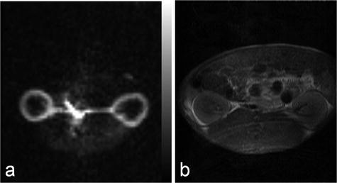
Fig. 9.

Renal cortical blood flow map (a) and the corresponding proton image (b) obtained in a rabbit.

2.4 Summary

In this section, MR applications of hyperpolarized agents within the field of angiography, perfusion, and interventional applications, have been reviewed.

The main aspects to be aware of are the following:

The character of hyperpolarized MR agents enables background-free angiographic and perfusion MR imaging.
The catheter, during an interventional procedure, may be visualized using a flowing hyperpolarized MR agent.
The MR signal is affected by the irreversible decay of the non-equilibrium polarization both due to locally varying T ₁ and the influence of RF pulses during the acquisition of dynamic images. The models that are used to extract perfusion information need to be adapted accordingly.
It is possible to quantify, e.g., cardiac or renal perfusion following intravenous injection of a hyperpolarized agent.

3 Metabolic Applications

3.1 Introduction

Most hyperpolarized MRI (metabolic MR) has been performed with [1-¹³C]pyruvate (62–64). Several other agents have been investigated and will be referenced in this chapter. However, the biochemistry of pyruvate serves as a good introduction to the field of metabolic MR. Pyruvate is a substance that is at a central crossroad of energy metabolism (65), Fig. 10. Pyruvate is reduced to lactate by the coenzyme NADH, in the reaction catalyzed by the enzyme lactate dehydrogenase (LDH). The resulting NAD⁺ is reestablished in the glycolytic pathway, which is an important source of ATP and also of biosynthetic intermediates. Oxidation of NADH by pyruvate allows the glycolytic pathway to produce ATP under anaerobic conditions, which is particularly important in tumors, which often have a poor and rapidly fluctuating blood supply and as a consequence are often hypoxic (66). Pyruvate can also be transaminated to form alanine in the reaction catalyzed by alanine aminotransferase (ALT). The source of the amino group for this reaction is glutamate. The reaction is particularly important in muscle, where, during fasting, amino groups resulting from protein degradation in the muscle are incorporated into alanine, which then passes via the circulation to the liver, where it is used to make glucose in the pathway of gluconeogenesis. The reactions catalyzed by LDH and ALT are thought to be near to equilibrium in most tissues and therefore these enzymes can catalyze rapid exchange of the ¹³C label in [1-¹³C]pyruvate with lactate and alanine respectively (67, 68). Pyruvate can also be oxidatively decarboxylated to produce acetyl CoA and ¹³CO₂ in the reaction catalyzed by pyruvate dehydrogenase (PDH). This irreversible reaction commits the carbon skeleton of pyruvate to oxidation in the tricarboxylic acid (TCA) cycle to form CO₂ and H₂O. The resulting reduced coenzymes, NADH and FADH₂, donate their electrons in the electron transport chain on the inner mitochondrial membrane to drive ATP synthesis. This is a fundamental energy process in all tissues, particularly those with a high energy demand, such as the heart. The NMR spectrum of these intermediates is shown in Fig. 10 and the chemical shifts are given in the figure legend.

Fig. 10.

Key metabolic pathways of pyruvate and illustration of isotopic labeling of metabolites. The labeled positions of the involved metabolites are highlighted by the gray circular shade. An in vivo 13C NMR spectrum of the metabolites is shown with molecular assignments. Chemical shifts (Ref. (99)) referenced to dioxane (external standard, 67.4 ppm) are CO₂ (124.5 ppm, not seen in spectrum), HCO₃ (160.9 ppm), pyruvate C-1 (170.6 ppm), lactate C-1 (183.2 ppm), alanine C-1 (176.5 ppm), and pyruvate hydrate C-1 (179.0 ppm).

It has been shown that pyruvate (and lactate) can enter cells by three different routes (69):

Transport on a specific H⁺-monocarboxylate transporter (MCT)
Through exchange for another anion
Free diffusion of the undissociated acid

These processes are tissue specific and differ in their kinetic properties (70). Ninety percent of the pyruvate and lactate transport is facilitated by MCTs. Lactate and pyruvate transport across the plasma membrane of liver cells has been studied in the isolated perfused liver, the liver in situ, freshly isolated and cultured hepatocytes, and plasma membrane vesicles (70). The maximum rate of influx of lactate at 37°C was found to be 50 nmol/min per μL of intracellular volume. Studies have shown that pyruvate is transported more rapidly than lactate. The sarcolemmal pyruvate uptake in cardiomyocytes varies exponentially with the extracellular pyruvate concentration. Besides the H⁺-linked carrier system, lactate appears to enter muscle cells quite rapidly by free diffusion of the undissociated acid at high concentrations (>10 mM). Brain capillary endothelial cells provide a barrier (the blood–brain barrier, BBB) for the exchange of solutes between the blood and cerebrospinal fluid. Lin et al. (71) found a wide distribution of several MCT isoforms in human tumor cell.

Lactate is not further metabolized in mammalian cells. Excess lactate is transported out of the cells and with the blood to the liver, where it is converted back to pyruvate and then into glucose by the gluconeogenic pathway. Thus, the liver restores glucose necessary for other organs to derive ATP from glycolysis. This constitutes the Cori cycle (65). Some cells, particularly cardiac, are highly permeable to lactate and pyruvate and since well oxygenated, can convert lactate back to pyruvate for further metabolism in the TCA cycle. Therefore, a contribution from inflow of [1-¹³C]lactate signal from the blood cannot be excluded and may contribute to the lactate signal observed in a particular region.

The NMR signal involved in these metabolic processes can be modeled by first-order rate equations (72, 73). The pyruvate-to-lactate exchange is considered as an example.

$\begin{array}{l} \dfrac{{{\textrm{d}}{L_z}}}{{{\textrm{d}}t}} = - {R_{\textrm{L}}}({L_z} - {L_\infty }) + {k_{\textrm{P}}}{P_z} - {k_{\textrm{L}}}{L_z} \\ \dfrac{{{\textrm{d}}{P_z}}}{{{\textrm{d}}t}} = - {R_{\textrm{P}}}({P_z} - {P_\infty }) + {k_{\textrm{L}}}{L_z} - {k_{\textrm{P}}}{P_z} \\ \end{array}$

([7])

where L _zand P _zare the lactate and pyruvate magnetizations respectively. L _∞ and P _∞ can usually be taken as zero since the thermal equilibrium polarization is lower by many orders of magnitude over the initial pyruvate polarization. R _L,P are the effective relaxation rates for the two molecules. The effective relaxation rate is the sum of the longitudinal relaxation rate, $T_{L,P}^{ - 1}$ , and the depolarization due to the radio-frequency pulses

${R_{{\textrm{L,P}}}} = \frac{1}{{T_{{\textrm{L,P}}}^1}} - \frac{{\ln \cos \alpha }}{{\Delta t}}$