Fig. 1.
Diagram of a spoiled, bright-blood gradient echo cine sequence frequently used in murine MRI: after the detection of the R-wave in the ECG, the same k-space line is acquired repeatedly with a constant value for the phase-encoding gradient. The number of frames N per cardiac cycle depends on the sequence timing and the heart rate of the animal and ranges between 15–30 frames. The illustrated scheme is repeated in the next cardiac cycle with a different value for the phase-encoding gradient. Thus, the product of number of phase-encoding steps times number of averages is the number of cardiac cycles that are required in total to obtain a full cine data set for one slice. If respiratory gating is employed, the scheme is interrupted during respiration (with or without steady-state maintenance) and the imaging time is prolonged. (Taken from Ref. (22), originally published by BioMed Central).
2.2 Animal Handling
1.
Standard anaesthesia set-up, comprising oxygen supply, vaporizer, anaesthetic chamber and scavenging unit with absorbers for isoflurane (see Note 8).
2.
Dedicated animal cradles, optimized in diameter and length, to maintain stable animal physiology throughout an experiment. The animal cradle should be comprised of a heating blanket to maintain the core body temperature at 37°C, a nose cone for continuous delivery of the anaesthetic and a scavenging line for anaesthetic gas recovery. Additional lines may be required if cardiac-stimulating drugs such as dobutamine, or MR contrast agents need to be administered.
3.
Ophthalmic lubrication (e.g. Viscotears, Novartis) in order to keep the eyes moist throughout the procedure as the eye closure reflex is suppressed during anaesthesia.
4.
Surface-mounted, or needle electrodes (∼25 gauge) inserted subcutaneously into the forelimbs to derive cardiac signal (see Note 9).
5.
Pressure pad to detect respiratory motion.
6.
Gating and monitoring device (see Note 5).
7.
Tools, such as a pair of tweezers and scissors.
8.
Consumables, such as gauze, (surgical) tape, gloves, isoflurane and isoflurane absorbers, saline.
9.
Heat pad for recovery.
2.3 Post-processing
1.
Computer to perform off-line data analysis.
2.
Off-line analysis may require additional software (typically MATLAB (The MathWorks, Natick, US) or IDL (ITT Visual Information Solutions, Boulder, US) to read MR data in the specific scanner format (raw or image data), process and/or convert them into a suitable image format (such as TIFF or JPEG).
3.
Analysis software, for example Amira (licensed – http://www.amiravis.com/) or ImageJ (free – http://rsb.info.nih.gov/ij/).
3 Methods
The overall procedure for assessing cardiac function can be divided into the following six steps:
1.
Preparation of the animal and positioning in the magnet with the heart in the isocentre of the RF-coil/gradients.
2.
Scan preparations, including tuning and matching the coil (if applicable), (slice-selective) shimming and RF-power calibration.
3.
Scouting for the short- and long-axis views.
4.
Multi-slice cine-MRI in short-axis orientation.
5.
Post-experimental procedures including animal recovery.
6.
(Off-line) data analysis.
3.1 Preparing the Set-Up
1.
Check isoflurane level at the vaporizer and the O2-level at the gas cylinder and refill/replace if required.
2.
Turn on the monitoring and recording device.
3.
Put some tissue into the anaesthetic chamber and open the valve in the gas line for filling the anaesthetic chamber.
4.
Connect animal handling with gas lines and electrical connections (i.e. ECG etc.).
5.
Mount appropriate cradle to animal handling system.
6.
Verify that ECG electrodes and pressure pad are sensitive.
7.
Switch on the heater and pre-heat the animal cradle.
8.
Cut sufficient number of tape strips of different lengths required during preparation and wet a small piece of gauze.
9.
Insert the corresponding RF probe into the magnet and connect it up.
10.
Set up experiment at the console computer by creating new study, selecting correct gradient and RF coil (where applicable) and provide scan-specific information, such as orientation, animal id, gender and purpose of experiment. Load the protocol for the first scan (see Section 3.3).
3.2 Animal Preparation
1.
Fill the anaesthetic chamber (O2 flow 4 L/min, isoflurane 4% for 4 min). Operate scavenging unit connected to the anaesthetic chamber in order to provide a homogeneous concentration of isoflurane in the chamber.
2.
Put the animal into the chamber until it is deep under anaesthesia (see Note 10).
3.
Reduce the oxygen flow to 1.5 l/min and the isoflurane concentration to 2.5% and start flushing the gas lines to the animal cradle.
4.
Weigh the animal and place it prone into the cradle with the nose into the cone. If tooth bars are available, hook it up to the front tooth and pull it back so that the nose is secured in the nose cone.
5.
Turn off the gas flow to the anaesthetic chamber.
6.
Connect the animal to the ECG electrodes; in case of needle electrodes carefully insert the needles subcutaneously into the front limbs and fix them with tape.
7.
Start recording the ECG trace. It is important to get optimal coupling between the animal and the electrodes. Sensitivity that is lost in first place can never be gained back!
8.
If applicable, ensure that the upper torso is resting on the surface coil(s).
9.
Place the respiratory pad below the abdomen of the animal (see Note 11).
10.
Tape down the front limbs on the side or the top of the nose cone; try to minimize the loop area that is formed by the limbs and the electrodes (this will minimize future problems related to gradient interference with the ECG) (see Note 12).
11.
Put ointment on both eyes, place a wet piece of gauze over the eyes and secure it with tape.
12.
Put a strip of tape loosely across the lower part of the back.
13.
Cover the animal with a lid and secure the lid.
14.
Reduce the isoflurane concentration to 1–1.5%.
3.3 Preparing the MR Scans
3.3.1 General
1.
Adjust and set the frequency.
2.
Adjust amplification of physiological signals (i.e. ECG and respiration) at the monitoring device and set trigger levels appropriately. Where applicable, adjust the window length for respiratory gating.
3.
SCAN_1: Run the scouting sequence consisting of three orthogonal planes, i.e. axial, sagittal and coronal orientations, respectively (Fig. 2).
4.
Reposition the animal and re-run if required.
5.
SCAN_2: If the heart is approximately in the centre of the coil(s), load and run the second scout consisting of four axial slices (gap 1–2 mm – Fig. 3).
6.
Tune and match the RF coil(s).
7.
Perform the shim procedure.
8.
Re-adjust the frequency.
9.
Perform power calibration.

Fig. 2.
Three orthogonal scout images. (a) Coronal, (b) sagittal and (c) axial orientation. Scale bar: 5 mm.
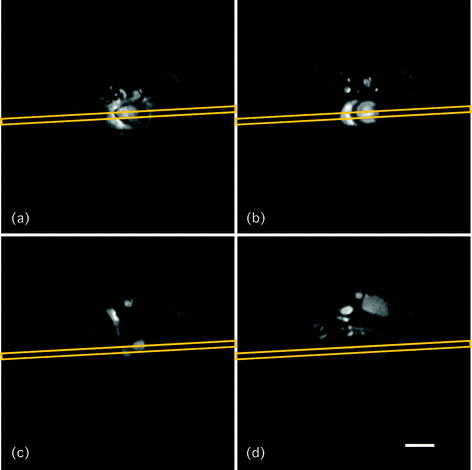
Fig. 3.
Axial scout scan. Four axial slices (thickness 1 mm, gap 2 mm) are acquired as the second scout scan, using a segmented GE sequence. The grey boxes in (a)–(d) show the orientation of the next, coronally placed scout scan (referred to as SCAN_3). Scale bar: 5 mm.
3.3.2 Scouting for Short-Axis
1.
2.
3.
SCAN_5 – short-axis orientation: Starting from ‘SCAN_3’, rotate the imaging slice by 90° (dashed light grey box in Fig. 4a); load ‘SCAN_4’ as reference and turn the imaging slice roughly perpendicular to the long-axis of the heart (dashed light grey box in Fig. 4b). It is recommended to set the correct field of view prior to running this scan (i.e. typical FOV 2.56–3 cm). Shift slice in plane so that the animal is fully contained. Swap read-out and phase encoding directions if required. The result (i.e. ‘SCAN_5’) is shown in Fig. 4c.
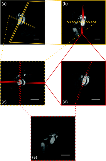
Fig. 4.
Illustration of how to obtain cardiac relevant views. Starting from (a) coronally orientated slice (SCAN_3), the next, more sagittally orientated view (SCAN_4 – shown in (b)) is obtained by cutting orthogonally through the outflow tract and the apex of the left ventricle of SCAN_3 as indicated by the solid light grey box in (a). (c) Short-axis scan (SCAN_5), obtained by placing the slice perpendicular to SCAN_3 and SCAN_4, respectively (light grey dashed boxes in (a, b)). The dark grey box in (b, c) indicates the slice position for obtaining the long-axis four-chamber view (SCAN_LA4c). (d) Longitudinal scan SCAN_LA4c. The dashed dark grey box in (c, d) illustrates the orientation to obtain the long-axis two-chamber view (SCAN_LA2c), which is depicted in (e). Note that FOV for images (c–e) is reduced (i.e. 25.6 × 25.6 mm versus 40 × 40 mm in (a, b)). Scale bars: 5 mm.
3.3.3 Running the Functional Study
1.
Load the cine protocol, import the slice orientation from the scan ‘SCAN_5’.
2.
Specify the number of frames according to the heart rate and the repetition time (take a delay of 10–20 ms at the end of the cine train into consideration to allow for variations in heart rate during the scan).
3.
Modify the slice offset for each scan to cover the heart from base to apex as shown in Fig. 5. Where applicable, update heart rate in the software and respiratory window length on the gating device.
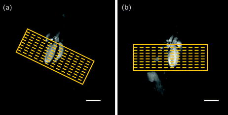
Fig. 5.
Multi-slice stack. The heart is covered from base to apex with multiple contiguous slices as indicated on (a) SCAN_3 and (b) SCAN_4, respectively. Scale bars: 5 mm.
3.3.4 Scouting for Long-Axis
1.
SCAN_LA4c – four-chamber long-axis: Starting from ‘SCAN_3’, place the imaging slice perpendicular to ‘SCAN_4’ through the base and the apex of the heart (dark grey rectangle in Fig. 4b) to cut through both, right and left ventricle in the short-axis scan (‘SCAN_5’) as indicated by the dark grey box in Fig. 4c. The resulting long-axis four-chamber (i.e. ‘SCAN_LA4c’) is shown in Fig. 4d.
2.
SCAN_LA2c – two-chamber long-axis: Starting from ‘SCAN_LA4c’, rotate the imaging slice by 90° on the reference image ‘SCAN_5’ and angulate it to section through the apex and outflow tract on ‘SCAN_LA4c’ (dark grey dashed boxes in Fig. 4c, d). The resulting two-axis four-chamber (i.e. ‘SCAN_LA2c’) is shown in Fig. 4e.
3.3.5 Scouting for Right-Ventricular Function Analysis
Due to the difference in geometry between the right and left ventricles, a slightly modified procedure is required to assess right ventricular function:
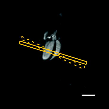

Fig. 6.
Right-ventricular function analysis. The slice orientation for assessing right ventricular function is orthogonal to the septum (solid box) rather than the long-axis of the left ventricle (dashed box). Scale bar: 5 mm.
3.4 Post-experimental Procedures
1.


Take the animal handling unit out of the magnet.
Stay updated, free articles. Join our Telegram channel

Full access? Get Clinical Tree


