The normalization takes into account that small signal differences can easily be masked when the overall signal intensity is high. It should be kept in mind that the ability to delineate two tissue structures also depends on the signal-to-noise ratio (SNR) of an image. The SNR is defined by the mean signal in a region of interest (ROI) normalized by the standard deviation (SD) of the background noise (Fig. 1).
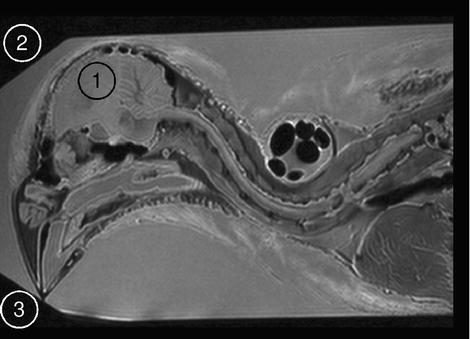
Fig. 1.
Definition of SNR in an MRI scan. The average signal in a region of interest (ROI 1), here in the brain of a fixed zebra finch specimen, is divided by the standard deviation in an image region devoid of spins, but inside the FOV (ROI 2 and ROI 3). To minimize systematic noise sources, noise is taken from several ROIs.
A high SNR value is no guarantee to delineate two different tissues when the signal intensities in the two ROIs are practically the same. On the other hand, a measurable signal difference that is on the same order as the noise of the data makes it also difficult to identify different structures – the contrast between two pixels might be reasonable but it does not mean anything if it does not stand out from the dynamic range of the noise. The introduction of the so-called contrast-to-noise ratio (CNR) therefore becomes increasingly popular (1). However, the usefulness of this quantity in terms of an objective measure is not generally accepted since the ability to discriminate details from the noise also depends on the individual visual reception by the observer.
The great advantage of MR imaging is the variety of parameters to generate contrast. Compared to X-ray imaging, where the contrast is solely based on the electron density of the material that causes an attenuation of the radiation that propagates through the tissue, MR signals are not exclusively determined by the density distribution of nuclear magnetic moments. This density depends on the concentration of the molecules that comprise the MR-sensitive nuclei. Since most MR images are based on the detection of hydrogen nuclei (i.e. protons), the proton density according to the water and fat concentration of the tissue is just one intrinsic contrast parameter (other molecules are practically not directly detectable; see Note 1). Beyond this unchangeable parameter, the pulse sequences in MR imaging can be used to actively manipulate the detectable magnetization. This precise manipulation is achieved during the following steps that characterize every MR experiment:
radiofrequency (rf) excitation of the system to generate detectable magnetization
evolution of the magnetization that drives the system back towards its thermodynamic equilibrium
encoding of the spatial information and readout of the manipulated magnetization
These three steps influence each other, especially since many MRI techniques are based on a repetitive acquisition of data, thus making the detected magnetization depend on the previous cycle of the experiment. We have to distinguish between two types of magnetization in order to understand the generation of contrast.
Longitudinal magnetization, which arises when the sample reaches its thermodynamic equilibrium in the external magnetic field and which is aligned with the latter. Longitudinal magnetization does not induce a detectable signal but can be conceived as the reservoir that is available for each rf excitation to generate detectable magnetization. The course of the MR experiment will influence the amount of this reservoir since each rf excitation can use up more or less of the available magnetization (see Note 2).
Transverse magnetization, which is generated by manipulating longitudinal magnetization with a short rf pulse. The so-called flip angle indicates how much the longitudinal magnetization is tipped off the z-axis, thereby producing a transverse component in the xy-plane (Fig. 2). This one precesses around the external field, thus inducing a detectable AC voltage signal in the detection antenna. It is this magnetization that is controlled during the spatial encoding by means of additional rf and magnetic field pulses and that decays to a certain extent before and during detection.
Fig. 2.
Various scenarios for conversion of longitudinal into transverse magnetization. (a) Thermal equilibrium with no detectable transverse component. (b) Small tip angle excitation that reduces the population difference between the two energy levels and generates a small FID signal. (c) A 90° excitation that causes equal population (so-called saturation) and the maximum available FID signal. (d) Inversion experiment with no detectable FID signal.
Each rf pulse represents a perturbation of the system which is followed by relaxation processes of the magnetization back to its thermal equilibrium. These processes are governed by inter-nuclear and inter-molecular mechanisms which depend on the physico-chemical environment of the spins (2). It is therefore possible to differentiate various types of tissue and visualize abnormal areas because of the underlying differences in relaxation. The reader should realize that these processes occur on a scale that is much smaller than the eventual image resolution.
In addition to the initial equilibrium magnetization (determined by the proton density, PD), all the three steps mentioned above have an influence on the two types of magnetization because they determine the initial disturbance of the system and the subsequent schedule of relaxation events. Hence, the interplay of sequence timing and relaxation mechanisms contributes to image contrast.
1.2 General Considerations on Image Quality
It should be mentioned at this point that the multi-dimensional parameter space for MRI contrast generation is in general accompanied by a trade-off between image quality in terms of SNR, spatial resolution and acquisition speed, i.e. temporal resolution. Several acquisition parameters influence the final result (see Note 3). Besides the sequence timing that controls influence of relaxation mechanisms, the following parameters are also important:
Field of view
Matrix size (i.e. the number of pixel elements)
Slice thickness
Number of averages
Receiver bandwidth
The first three are geometric parameters that simply determine how many spins contribute to the signal in each subunit of the image. Better spatial resolution therefore cuts down the received induction signal per pixel. This can be compensated for by signal averaging since the real signal accumulates linearly whereas contributions to the noise partially cancel each other and increase only with the square root of the number of acquisitions. Hence, the number of acquisitions has to be quadrupled to maintain a certain SNR when the spatial resolution improves by a factor of 2 (e.g. halving the slice thickness or changing from 100 to 50 μm in one dimension). The receiver bandwidth must be large enough to allow for recording of all frequency components from the entire field of view (see Note 4), but the acquisition of noise also increases with the square root of this parameter.
Although strong gradients are a prerequisite to improve spatial resolution for resolving small structures, they are, however, useless if they are not paired with rf-receiving hardware that ensures the necessary sensitivity to detect a decreasing number of spins. Hence, the detectable SNR at a certain spatial resolution is an important parameter to judge the quality of an MRI system. The achievable resolution depends on the object that is imaged and on the optimized detectors. The state of the art is reflected in the examples given in the following chapters of this book (3). Current progress is also based on a new type of coils that reduces noise by cooling the rf circuits with helium or liquid nitrogen. These so-called cryo-probes gain a factor of 2–3 in sensitivity that can be used to improve spatial or temporal resolution (4).
1.3 T1 Relaxation
1.3.1 Physical Background
T 1 relaxation is the process that is responsible for recovery of longitudinal magnetization after excitation by an rf pulse. Since longitudinal magnetization is defined by the difference of spins in parallel and antiparellel orientation, it is related to the energy of the spin system and the corresponding relaxation is the recovery from an excited state back to thermal equilibrium through loss of energy. This is an exponential process (see Fig. 3) that is characterized by the time constant T 1 (see Note 5). The full range of relaxation occurs after an inversion pulse with a zero passage at  (inversion-recovery experiment). Almost complete recovery after maximum signal generation by a 90° pulse that leaves no longitudinal magnetization (the so-called saturation-recovery experiment) is achieved after ca. 3T 1.
(inversion-recovery experiment). Almost complete recovery after maximum signal generation by a 90° pulse that leaves no longitudinal magnetization (the so-called saturation-recovery experiment) is achieved after ca. 3T 1.Fig. 3.
Different longitudinal relaxation scenarios. (a) recovery after small tip angle excitation. (b) Saturation recovery for two different relaxation times T 1. (c) Inversion recovery for a fast and a slow component, illustrating the expected signal difference when the slow component has its zero-passage.
Exchange of energy occurs with the neighbouring nuclei and molecules that are sometimes summarized in the generalized term “lattice” (see Note 6). T 1 relaxation is therefore also called spin–lattice relaxation. The source of the relaxation process is the fluctuating fields caused by the sum of the fields attributed to surrounding electrons and nuclei. The detected nuclei experience an oscillating field due to molecular tumbling. If the spectrum of the fluctuations caused by the surrounding molecules contains components at the NMR resonance frequency ω (ca. 50–500 MHz) or 2ω it can absorb energy from the detected spin system and therefore drive the system back into its thermodynamic equilibrium. Components contributing at 2ω are actually weighted four times as much as components at ω (2). T 1 relaxation increases as the molecular mobility decreases but becomes very slow again for extreme conditions such as those in solids. Therefore, areas with less restriction in molecular tumbling (such as the cerebrospinal fluid) are characterized by long T 1 values whereas tissue rich in microstructure (e.g. muscle) exhibit fast T 1 relaxation. Some examples are given in Table 1.
Tissue | T 1 [ms] | T 2 [ms] |
|---|---|---|
Grey matter | 1900 | 40 |
White matter | 1700 | 32 |
Muscle | 2100 | 20 |
Fat | 850 | 30 |
1.3.2 Repetitive Nature of Data Acquisition: How to Use T1 Relaxation
Most standard MR-imaging sequences require a repetitive excitation of the magnetization because the spatial encoding is not done in a single shot (5). The raw data space from which the image is finally computed is filled up in a line-by-line scheme, thus introducing a dependence of each line’s signal intensity on the previous acquisition step. Sufficient spatial resolution often requires the acquisition of tens to hundreds of lines in raw data space and the desired acquisition time ranges from the sub-second regime to the order of several minutes or even hours. This combination yields repetition times (TR) that are on the order of T 1 relaxation and therefore automatically allows using this effect for generation of contrast by adjusting TR properly.
A fast repetition of the pulse sequence can “saturate” the spin system (see Note 7) and therefore impair the subsequent generation of transverse magnetization to encode the image information. In contrast, very slow repetition will eliminate the relaxation influence and the differences in T 1 between various tissues fade out, thus yielding a method to eliminate this contribution to emphasize other types of contrast.
1.3.3 Manipulating T1 Relaxation: Contrast Agents and External Field
The fact that relaxation depends on the fluctuating magnetic fields experienced by the nuclear spins introduces the opportunity to enhance natural T 1 relaxation by introducing additional magnetic moments that influence the detected protons in water (and fat) molecules. Such magnetic moments are provided by unpaired electrons, e.g. in Fe3+, Mn2+ or Gd3+ ions (6). The paramagnetic effect from electron-rich systems like lanthanide complexes is especially efficient since the magnetic moment of each electron is ca. 600 times larger than that of protons. Gadolinium, e.g. has seven unpaired electrons that alter the relaxation of adjacent protons very efficiently. The element itself is toxic and has to be made harmless by complex formation, e.g. with hydrophilic poly(aminocarboxylate) ligands. One or two coordination sites are occupied by water molecules (7) that are temporarily bound to the Gd ion and therefore experience efficient dipolar interactions with the electron spins. Such interactions fall off rapidly with increasing distance but water molecules in the inner hydration shell of these complexes are also affected to some extent by relaxation effects.
Such complexes influence both T 1 and T 2 relaxation but the dominant effect is shortening the slower longitudinal relaxation. Gd chelates therefore cause bright signal contributions in T 1-weighted MR images (so-called positive contrast). This can be used to increase contrast between two types of tissue or allow retaining contrast while speeding up the acquisition by using shorter repetition times. The effect can be amplified even more by “adjusting” the correlation time of such molecules: macromolecular contrast agents have a higher relaxivity due to their reduced tumbling rate and can therefore be detected at lower concentrations (see Note 8). In any case, this type of contrast agents only affects areas where it is directly accessible since the water needs to get close to the paramagnetic centre.
Since there is no way to reduce the number of fluctuating magnetic moments in tissue, a reduction of T 1 relaxation can only be achieved by reducing the matching frequency components in the above-mentioned range of fluctuations. By increasing the field strength B 0 of the scanner system, the resonance frequency of the detected water molecules is shifted against the fixed spectrum of field fluctuations due to molecular motion. Resonant contributions are less pronounced and T 1 relaxation times increase when switching from standard clinical field strengths of 1.5–3 T to modern high-field scanners of 7 T or more (8).
1.3.4 Practical Considerations: Acquisition Time
Several experimental setups require a certain temporal resolution for consecutive imaging or are subject to other constraints that determine an upper limit for the total acquisition time. Since longitudinal relaxation is a property of the tissue that can be manipulated by contrast agents only to some extent, choice of the suitable imaging sequence can depend on the speed of the encoding scheme. The total acquisition time is given by the product of the repetition time (TR), the number of phase encoding steps (N ph) and the number of acquisitions (N aq; see Note 9):
For some applications, it is therefore necessary to use sequences that achieve the desired contrast even for relatively short TR, i.e. acquisition schemes that minimize the disturbance of the longitudinal magnetization.
It should be mentioned at this point that T 1 relaxation of protons is relatively favourable for most in vivo applications (see Table 1). Other nuclei such as 31P have longer relaxation times (9) (see Note 10). Given the fact that the relative sensitivity for such nuclei is much smaller (see Note 11), small flip angle excitations often yield insufficient signal and the required 90° excitation is then related to very long TR or substantial saturation effects. This aggravates the problem for many nuclei other than 1H to collect MRI datasets in a reasonable amount of time.
1.4 T2 Relaxation
1.4.1 Physical Background
The signal strength induced by the precessing transverse magnetization depends on the phase coherence among the different spin packages. Loss of this coherence is called transverse relaxation. The amplitude of the vector sum of all magnetizations is decreasing exponentially with a time constant T 2 (Fig. 4a, b). The process is also called spin–spin relaxation and is not related to loss of energy (like T 1 relaxation). Compared to longitudinal relaxation, this process occurs more rapidly because additional mechanisms contribute. Microscopic processes such as interactions with the local magnetic fields of neighbouring nuclei are governed by the molecular tumbling rate and the spectral density of different tumbling modes. Transverse relaxation is influenced by spectral components at ω, 2ω (less weighted than the previous one) and low-frequency components (intermediate weight) (2). Rapid motion causes averaging of spin–spin interactions over time and makes such processes less efficient, thereby slowing down T 2 relaxation. Relaxation times for free water molecules are therefore relatively long (ca. 3 s and are mostly independent of the magnetic field strength) whereas T 2 values for macromolecules bound to cell membranes are on the order of a few microseconds only. In the latter case, relaxation is more efficient because of the longer “contact time” between molecules. Skeletal muscle tissue is an example for tissue with relative short T 2 values (see Table 1).
Fig. 4.
Different scenarios for transverse relaxation. (a) FID signal showing T 2 relaxation during signal acquisition. (b) Two T 2 decays and corresponding signal difference illustrating the optimum timing for maximum contrast. (c) FID and echo formation with two different echo times TE.
Very rapid T 1 relaxation usually does not impose a problem (in fact, it is sometimes desired and generated with suitable contrast agents); however, extensive T 2 relaxation can impede acquisition of sufficient signal intensity even for short echo times. The scanner hardware is limited in terms of arbitrarily fast pulse sequences due to minimum times for switching the rf and gradient pulses on and off. Hence, some nuclei with very short T 2 (e.g. sodium or even protons in case they are in a macromolecular environment) are hard to detect and give only small signal contributions.
1.4.2 T2* Relaxation
Loss of phase coherence between the different magnetizations within a sample happens not only as an intrinsic process in terms of spin–spin interactions, it is also a consequence of local field inhomogeneities ΔB that cause small differences in precession frequencies of different spin packages. This process therefore enhances transverse relaxation. It is called T 2* relaxation and happens on a timescale faster than pure T 2 processes. T 2 and T 2* relaxation rates, i.e. the inverse of the relaxation times, are linked through the following equation:
Since we deal with the sum of the rates, the differences between T 2 and T 2* are less pronounced for fast-relaxing tissue for a given field inhomogeneity. In general, imperfections of the magnetic field increase with the distance from the centre of the magnet (the so-called iso-centre or sweet spot; see Note 12). Inhomogeneities can also be caused by exogenous para- or ferromagnetic material (see Note 13).
Related posts:
Stay updated, free articles. Join our Telegram channel

Full access? Get Clinical Tree


