Magnetic resonance (MR) spectroscopy offers a noninvasive means of assessing in vivo brain metabolites that shed light on cellular concentrations, cell function and dysfunction, cellular energetics, presence of ischemia, and presence of necrosis, among others. Studies obtained at higher field strengths are evolving toward sampling of smaller tissue volumes, greater signal-to-noise ratio, and higher metabolic spatial resolution. This article discusses the usefulness, from the clinical standpoint, of MR spectroscopy in various disorders. However, to be valid and significant the results of MR spectroscopy should always be correlated with their imaging counterparts.
Key points
- •
Magnetic resonance (MR) proton spectroscopy is a technique which mainly provides biological information regarding cellularity, energy, neuron viability, necrosis and ischemia.
- •
MR spectroscopy is ideal to assess the limits of brain tumors when planning surgery.
- •
MR spectroscopy allows identification of some metabolic disorders guiding further laboratory analysis.
Introduction
Magnetic resonance (MR) spectroscopy is an analytical method used in chemistry that enables the identification and quantification of metabolites in samples. It differs from conventional MR imaging in that spectra provide physiologic and chemical information instead of anatomy.
MR spectroscopy and MR imaging have their origin in nuclear magnetic resonance (NMR). NMR was first described in 1946 simultaneously by the Nobel Prize winners Edward Purcell, from Harvard University, and Felix Bloch, from Stanford University. At that time, NMR was used only by physicists for purposes of determining the nuclear magnetic moments of nuclei. It was only in the mid 1970s that NMR started to be used in vivo, after Lauterbur, Mansfield, and Grannell introduced gradient into the magnetic field, enabling them to determine the location of the emitted signal and to reproduce it on an image. In vivo NMR was renamed MR imaging because the term “nuclear” had been consistently (but erroneously) associated with nuclear medicine. For the same reason, NMR spectroscopy used in vivo is now named MR spectroscopy. During the 1980s, the first MR imaging medical scanners became available for clinical use. Since then improvements have been made, especially in relation to higher field strengths.
MR spectra may be obtained from different nuclei. Protons ( 1 H) are the nuclei most used for clinical applications in the human brain, mainly because of their high sensitivity and abundance. The proton MR spectrum is altered in almost all neurologic disorders. In some diseases, proton MR spectroscopy ( 1 H-MRS) changes are very subtle and are not reliable without a statistical comparison between groups of patients. In these cases, 1 H-MRS is usually used for research. In clinical practice, 1 H-MRS is mostly used for more detailed analysis of primary and secondary brain tumors and metabolic diseases.
This article discusses the physical basis of 1 H-MRS, emphasizing the different techniques, the normal spectra in adults and children, its clinical applications, and the significance of brain metabolites under both normal and abnormal conditions, particularly in the evaluation of brain tumors.
Physical basis
Many nuclei may be used to obtain MR spectra, including phosphorus ( 31 P), fluorine ( 19 F), carbon ( 13 C), and sodium ( 23 Na). The ones mostly used for clinical MR spectroscopy are protons ( 1 H). The brain is ideally imaged with 1 H-MRS because of its near lack of motion (this prevents MR spectroscopy from being used in the abdomen and thorax without very sophisticated motion-reduction techniques). The hydrogen nucleus is abundant in human tissues. 1 H-MRS requires only standard radiofrequency (RF) coils and a dedicated software package. For nonproton MR spectroscopy, RF coils tuned to the Larmor frequency of other nuclei, matching preamplifiers, hybrids, and a broadband power amplifier are needed.
Different field strengths are used for conventional clinical MR imaging, ranging from 0.2 to 3 T. Because the main objective of 1 H-MRS is to detect weak signals from metabolites, a minimum of 1.5 T is advised. Units with higher field strength have the advantage of higher signal-to-noise ratio (SNR), better resolution, and shorter acquisition times, making the technique useful in sick patients and others who cannot hold still for long periods of time.
1 H-MRS is based on the chemical-shift properties of the atom. When a tissue is exposed to an external magnetic field, its nuclei will resonate at a frequency ( f ) that is given by the Larmor equation:
Because the gyromagnetic ratio (γ) is a constant of each nuclear species, the spin frequencies of certain nuclei ( f ) depend on the external magnetic field ( B 0 ) and the local microenvironment. The electric shell interactions of these nuclei with the surrounding molecules cause a change in the local magnetic field, leading to a change on the spin frequency of the atom (a phenomenon called chemical shift). The value of this difference in resonance frequency gives information about the molecular group carrying 1 H and is expressed in parts per million (ppm). The chemical-shift position of a nucleus is ideally expressed in ppm because it is independent of the field strength (choline, for example, will be positioned at 3.22 ppm at 1.5 or 7 T). The MR spectrum is represented by the x axis that corresponds to the metabolite frequency in ppm according to the chemical shift, and the y axis that corresponds to the peak amplitude.
Some metabolites such as lactate have doublets, triplets, or multiplets instead of single peaks. These peaks are broken down into more complex peaks and are explained by J-coupling, also named spin-spin coupling. The J-coupling phenomenon occurs when the molecular structure of a metabolite is such that protons are found in different atomic groups (eg, CH 3 – and CH 2 -). These groups have slightly different local magnetic fields, thus each 1 H resonates at a frequency that is characteristic of its position in the molecule, resulting in a multiplet peak.
Techniques
The 1 H-MRS acquisition usually starts with anatomic images, which are used to select a volume of interest (VOI), where the spectrum will be acquired. For the spectrum acquisition, different techniques may be used, including single-voxel and multi-voxel imaging using both long and short echo times (TE). Each technique has advantages and disadvantages, and choosing the right one for a specific purpose is important in improving the quality of the results.
Single-voxel spectroscopy
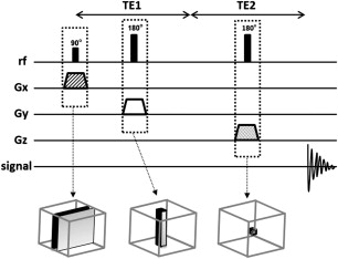
In single-voxel spectroscopy (SVS) the signal is obtained from a voxel previously selected. This voxel is acquired from a combination of slice-selective excitations in 3 dimensions in space, achieved when an RF pulse is applied while a field gradient is switched on. It results in 3 orthogonal planes whose intersection corresponds to the VOI ( Fig. 1 ).
One of two techniques is typically used for acquisition of SVS 1 H-MRS spectra: pointed-resolved spectroscopy (PRESS) and stimulated echo acquisition mode (STEAM). The most used SVS technique is PRESS. In the PRESS sequence, the spectrum is acquired using 1 90° pulse followed by 2 180° pulses, each of which is applied at the same time as a different field gradient. Thus, the signal emitted by the VOI is a spin echo. The first 180° pulse is applied after time TE1/2 from the first pulse (90° pulse), and the second 180° is applied after time TE1/2 + TE. The signal occurs after a time 2TE ( Fig. 2 ). To restrict the acquired sign to the selected VOI, spoiler gradients are needed. Spoiler gradients dephase the nuclei outside the VOI and reduce their signal.
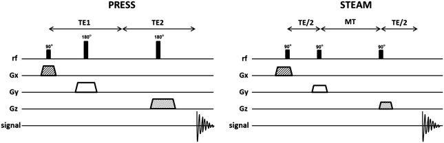
STEAM is the second most commonly used SVS technique. In this sequence all 3 pulses applied are 90° pulses. As in PRESS, they are all simultaneous with different field gradients. After time TE1/2 from the first pulse, a second 90° pulse is applied. The time elapsed between the second and the third pulse is conventionally called mixing time (MT), and is shorter than TE. The signal is finally achieved after time TE + MT from the first pulse (see Fig. 2 ). Thus, the total time for the STEAM technique is shorter than that for PRESS. Spoiler gradients are also needed to reduce signal from regions outside the VOI.
The STEAM sequence uses only 90° pulses, which results in 50% lower SNR than for PRESS. As described, the PRESS sequence is acquired using 2 pulses of 180°. The use of these 180° pulses results in a less optimal VOI profile and leads to a higher SNR. However, because the length of 180° pulses is longer than 90°, PRESS cannot be achieved with a very short TE. Another disadvantage of the PRESS sequence is the larger chemical-shift displacement artifact, which is described later in this article. Therefore, STEAM is usually the modality of choice when a short TE and precise volume selection is needed. Nevertheless, PRESS is the most used SVS technique because it doubles the SNR, which is an important factor that leads to better spectral quality.
Magnetic resonance spectroscopy imaging
MR spectroscopy imaging, also called spectroscopic imaging or chemical-shift imaging, is a multivoxel technique. The main objective of MR spectroscopy imaging is to simultaneously acquire many voxels and a spatial distribution of the metabolites within a single sequence. Thus, this 1 H-MRS technique uses phase-encoding gradients to encode spatial information after the RF pulses and the gradient of slice selection.
MR spectroscopy imaging is acquired using only slice selection and phase-encoding gradients, besides the spoiler gradients. A frequency encoding gradient is not applied. Thus, instead of the anatomic information given by the conventional MR imaging signal, the 1 H-MRS signal results in a spectrum of metabolites with different frequencies (information acquired from chemical-shift properties of each metabolite).
The same sequences used for SVS are used for the signal acquisition in MR spectroscopy imaging (STEAM or PRESS). The main difference between MR spectroscopy imaging and SVS is that, after the RF pulse, phase-encoding gradients are used in 1, 2, or 3 dimensions (1D, 2D, or 3D) to sample the k -space ( Fig. 3 ). In a 1D sequence the phase encoding has a single direction, in 2D it has 2 orthogonal directions, and in 3D it has 3 orthogonal directions.
The result of a 2D MR spectroscopy imaging is a matrix, called a spectroscopy grid. The size of this grid corresponds to the field of view (FOV) previously determined. In the 3D sequence, many grids are acquired within one FOV. The number of partitions (or voxels) of the grids is directly proportional to the number of phase-encoding steps. The spatial resolution is also proportional to the number of voxels in a determined FOV (more voxels give a better spatial resolution). However, for a larger number of voxels, more phase-encoding steps are needed, and this implies a longer time for acquisition. Spatial resolution is also determined by the size of the FOV (a smaller FOV gives better spatial resolution) and by the point-of-spread function (PSF).
PSF on an optical system is defined as the distribution of light from a single point source. For MR spectroscopy imaging, the PSF is related to voxel contamination with signals from adjacent voxels, also called voxel “bleeding.” This same effect corresponds to the Gibbs ringing artifact seen on conventional MR imaging. The shape of PSF is determined by the k -space sampling method and the number of phase-encoding steps. PSF can be avoided when more than 64 phase-encoding steps are applied, which leads to a scanning time not feasible in clinical practice. To reduce PSF, methods such as k -space filtering and reduction are used. For k -space reduction, the measured data are restricted to a circular (2D) or spherical (3D) region.
Another concern about MR spectroscopy imaging is the suppression of unwanted signals from outside the brain, particularly from the subcutaneous fat, because lipids have a much higher signal than brain metabolites. Because the FOV is always rectangular and does not conform to the shape of the brain, some techniques must be implemented to optimize the FOV. The use of outer-volume suppression (OVS) is the technique most used for this purpose.
All techniques that help optimize the MR spectroscopy imaging sequence by reducing voxel bleeding, and by increasing spatial resolution and the amount of phase encoding needed to acquire a 2D or 3D MR spectroscopy image, have a time cost. Therefore to minimize scan time without reducing quality, fast MR spectroscopy imaging techniques are used. A large FOV means a longer MR spectrum acquisition time. A simple way to reduce time is to use the smallest possible FOV consistent with the dimension of the object to be analyzed.
Reducing the k- space sampling by measuring the data inside a circular or spherical region instead of a rectangular one is another way to reduce scan time. Other techniques used for this purpose are turbo-MR spectroscopy imaging (using multiple spin echoes), multislice MR spectroscopy imaging, 3D echo-planar spectroscopic imaging, and parallel imaging methods. These techniques are beyond the scope of this article, and more details on these methods can be found elsewhere.
SVS versus MR spectroscopy imaging
SVS and MR spectroscopy imaging have advantages and disadvantages, depending on the specific purpose ( Table 1 ). The SVS technique results in a high-quality spectrum, short scan time, and good field homogeneity. Thus, SVS technique is usually obtained with short TE because longer TE has a decreased signal owing to T2 relaxation. SVS is used to obtain an accurate quantification of the metabolites.
| SVS | MR Spectroscopy Imaging |
|---|---|
| Short TE | Long TE |
| One voxel | Multivoxel |
| Limited region | Many data collected |
| Fixed grid | Grid may be shifted after acquisition |
| More accurate | Voxel bleeding |
| Quantitative measurement | Spatial distribution |
The main advantage of MR spectroscopy imaging is spatial distribution, compared with SVS that only acquires the spectrum in a limited brain region. Moreover, the grid obtained with MR spectroscopy imaging allows voxels to be repositioned during postprocessing. On the other hand, the quantification of the metabolites is not as precise when using MR spectroscopy imaging because of voxel bleeding. Therefore, MR spectroscopy imaging can be used to determine spatial heterogeneity.
Short TE versus long TE
1 H-MRS can be obtained using different TEs that result in distinct spectra. Short-TE studies (typically 20–40 milliseconds) have a high SNR and less signal loss because of T2 and T1 weighting. These short-TE properties result in a spectrum with more metabolites peaks, such as myoinositol and glutamine-glutamate ( Fig. 4 ), which are not detected with long TE. Nevertheless, because more peaks are shown on the spectrum, overlap is much more common, and care must be taken when quantifying the peaks of metabolites.
1 H-MRS spectra may also be obtained with long TEs, from 135 to 288 milliseconds. Long TEs have a poorer SNR; however, they have more simple spectra because of the suppression of some signals. Thus, the spectra are less noisy but have a limited number of sharp resonances. On 135- to 144-millisecond TEs, the peak of lactate is inverted below the baseline. This factor is important because the peaks of lactate and lipids overlap in this spectrum. Therefore, 135- to 144-millisecond TEs allow for easier recognition of the lactate peak (see Fig. 4 ) because lipids remain above the baseline. With a TE of 270 to 288 milliseconds there is a lower SNR and the lactate peak is not inverted.
Water Suppression
1 H-MRS–visible brain metabolites have a low concentration in brain tissues. Water is the most abundant, and thus its signal in the 1 H-MRS spectrum is much higher than that of other metabolites (the signal of water is 100,000 times greater than that of other metabolites). To avoid this high peak from water to be superimposed on the signal of other brain metabolites, water-suppression techniques are needed ( Fig. 5 ). The most commonly used technique is chemical-shift selective water suppression (CHESS), which presaturates the water signal using frequency-selective 90° pulses before the localizing pulse sequence. Other techniques sometimes used are variable pulse power and optimized relaxation delays (VAPOR) and water suppression enhanced through T1 effects (WET).
Postprocessing
Quantification and analysis methods of collected data are as important as the acquisition techniques used to obtain the spectra. Using an incorrect postprocessing method may lead to wrong interpretations. There are many postprocessing techniques that may be used before and after the Fourier transform (FT).
The properties of the spectrum can be manipulated using digital filters before the FT. Zero-filling, multiplication with a filter, eddy-current correction, and band-reject filters are some examples of postprocessing steps in the time domain. The use of zero-filling results in a higher digital resolution in the spectrum. Band-reject filters are used to remove residual water signal when the water-suppression technique used during signal acquisition does not completely eliminate it. Eddy-current correction is used to eliminate eddy-current artifacts (explained in the Artifacts section) using a reference signal such as unsuppressed water signal and applying a time-dependent phase correction. After the FT, in the frequency domain, phase and baseline correction are usually used. All these postprocessing methods may be used with SVS and MR spectroscopy imaging. However, because MR spectroscopy imaging uses phase-encoding gradients, other filters need to be applied before FT (eg, Hanning, Hamming, and Fermi filters).
Artifacts
1 H-MRS is prone to artifacts. Motion, poor water or lipid suppression, field inhomogeneity, eddy currents, and chemical-shift displacement are some examples of factors that introduce artifacts into spectra. One of the most important factors that predict the quality of a spectrum is the homogeneity of the magnetic field. Poor field homogeneity results in a lower SNR and broadening of the width of the peaks. For brain 1 H-MRS, some regions are more susceptible to this artifact, including those near bone structures and air-tissue interfaces. Therefore, placement of the VOI near areas such as inferior and anterior temporal cortices and orbitofrontal regions should be avoided. Paramagnetic devices also result in field inhomogeneity, leading to a poor-quality spectrum when the VOI is placed near them.
Eddy currents are caused by gradient switching. A transient current results in distortion of the peak shapes, making spectrum quantification difficult. This artifact is more commonly seen in older MR imaging units. However, even modern units produce smaller eddy-current artifacts, and eddy-current correction (used postprocessing) is needed.
Chemical-shift displacements correspond to chemical-shift artifacts on conventional MR imaging. The localization of the voxel is based on the precession frequency of the protons. Because this frequency is different for each metabolite, the exact position of each metabolite is slightly different. This artifact is larger with higher magnetic field strengths. To solve this problem, strong field gradients must be used for the slice selection.
Higher-Field 1 H-MRS
Higher-field MR imaging (3 T, 7 T, and above) is used in many centers mostly for research purposes. In the past decade 3-T MR imaging has started to be routinely used for clinical examinations, resulting in better SNR and faster acquisition time.
1 H-MRS at 3 T has a higher SNR and shorter acquisition time than when performed at 1.5 T. It had been assumed that SNR increases linearly with the strength of the magnetic field, but SNR does not double with 3-T 1 H-MRS because others factors are also responsible for the SNR, including metabolite relaxation time and magnetic-field homogeneity.
Spectral resolution is improved with a higher magnetic field. A better spatial resolution increases the distance between peaks, making it easier to distinguish between them. This aspect is important, particularly for resonances from coupled spins such as glutamate, glutamine, and myoinositol. However, the line-width of metabolites also increases at higher magnetic field because of a markedly increased T2 relaxation time. Thus, a short TE is more commonly used with 3 T. The difference in T1 relaxation time from 1.5 to 3 T depends on the brain region studied.
3-T 1 H-MRS is more sensitive to magnetic-field inhomogeneity, and some artifacts are more pronounced (eg, susceptibility and eddy currents). Chemical-shift displacement is also greater at 3 T, and this artifact increases linearly with the magnetic field.
Receiver coils have also improved. The use of multiple RF receiver coils for 1 H-MRS provides higher local sensitivity and results in a higher SNR. These coils also allow a more extended coverage of the brain.
Spectra
1 H-MRS allows the detection of brain metabolites. The metabolite changes often precede structural abnormalities, and 1 H-MRS can demonstrate abnormalities before MR imaging does. To detect these spectral alterations, it is fundamental to know the normal brain spectra and their variations according to the applied technique, patient’s age, and brain region.
1 H spectra of metabolites are shown on x and y axes. The x (horizontal) axis displays the chemical shift of the metabolites in units of ppm. The ppm increases from right to left. The y (vertical) axis demonstrates arbitrary signal amplitude of the metabolites. The height of metabolic peak refers to a relative concentration, and the area under the curve to metabolite concentration.
Long TE sequences result in less noise than short TE sequences, but several metabolites are better demonstrated with short TE. In 1.5-T MR scanners, long TE sequences (TE = 135–288 milliseconds) detect N -acetylaspartate (NAA), creatine (Cr), choline (Cho), lactate (Lac) and, possibly, alanine (Ala). Short TE sequences (TE = 20–40 milliseconds) demonstrate the metabolites seen with long-TE acquisitions and, in addition, lipids, myoinositol (Myo), glutamate-glutamine (Glx), glucose, and some macromolecular proteins ( Fig. 6 ).
Brain Metabolites
N -acetylaspartate
The peak of NAA is the highest peak in normal brain, assigned at 2.02 ppm. NAA is synthesized in the mitochondria of neurons, then transported into neuronal cytoplasm and along axons. NAA is exclusively found in the nervous system (peripheral and central), and is detected in both gray and white matter. It is a marker of neuronal and axonal viability and density. NAA can additionally be found in immature oligodendrocytes and astrocyte progenitor cells. NAA also plays a role as a cerebral osmolyte.
Absence or decreased concentration of NAA is a sign of neuronal loss or degradation. Neuronal destruction from malignant neoplasms and many white-matter diseases results in decreased concentration of NAA. By contrast, increased NAA indicates Canavan disease, although it may also be demonstrated in Salla disease and Pelizaeus-Merzbacher disease. NAA is not demonstrated in extra-axial lesions such as meningiomas or intra-axial ones originating from outside of the brain such as metastases, unless there is a partial volume effect with normal parenchyma.
Creatine
The peak of the Cr spectrum is assigned at 3.02 ppm. This peak represents a combination of molecules containing creatine and phosphocreatine. Cr is a marker of energetic systems and intracellular metabolism. The concentration of Cr is relatively constant, and it is considered a stable metabolite. It is therefore used as an internal reference for calculating metabolite ratios. However, there is regional and individual variability in Cr concentrations.
In brain tumors, the Cr signal is relatively variable (see later discussion). Gliosis may cause minimally increased Cr, owing to increased density of glial cells (glial proliferation). Creatine and phosphocreatine are metabolized to creatinine, then the creatinine is excreted via the kidneys. Systemic disease (eg, renal disease) may also affect Cr levels in the brain.
Choline
The Cho spectrum peak is assigned at 3.22 ppm and represents the sum of choline and choline-containing compounds (eg, phosphocholine). Cho is a marker of cellular membrane turnover (phospholipids synthesis and degradation) reflecting cellular proliferation. In tumors, Cho levels correlate with degree of malignancy reflecting cellularity. Increased Cho may be seen in infarction (from gliosis or ischemic damage to myelin) or inflammation (glial proliferation). For this reason, Cho is considered to be nonspecific.
Lactate
The Lac peak is difficult to visualize in the normal brain. The peak of Lac is a doublet at 1.33 ppm, which projects above the baseline on short/long TE acquisition and inverts below the baseline at TE of 135 to 144 milliseconds.
A small peak of Lac is visible in some physiologic states such as newborn brains during the first hours of life. Lac is a product of anaerobic glycolysis, so its concentration increases under anaerobic metabolism such as cerebral hypoxia, ischemia, seizures, and metabolic disorders (especially mitochondrial ones). Increased Lac signals also occur with macrophage accumulation (eg, acute inflammation). Lac also accumulates in tissues with poor washout such as cysts, normal-pressure hydrocephalus, and necrotic and cystic tumors.
Lipids
Lipids are components of cell membranes not visualized with long TE because of their very short relaxation time. There are 2 peaks of lipids: methylene protons at 1.3 ppm and methyl protons at 0.9 ppm. These peaks are absent in the normal brain, but presence of lipids may result from improper voxel selection, causing voxel contamination from adjacent fatty tissues (eg, fat in subcutaneous tissue, scalp, and diploic space).
Lipid peaks can be seen when there is cellular membrane breakdown or necrosis, such as in metastases or primary malignant tumors.
Myoinositol
Myo is a simple sugar assigned at 3.56 ppm. Myo is considered a glial marker because it is primarily synthesized in glial cells, almost only in astrocytes. It is also the most important osmolyte in astrocytes. Myo may represent a product of myelin degradation. Elevated Myo occurs with proliferation of glial cells or with increased glial-cell size, as found in inflammation. Myo is elevated in gliosis, astrocytosis, and Alzheimer disease (AD).
Alanine
Ala is an amino acid that has a doublet centered at 1.48 ppm. This peak is located above the baseline in spectra obtained with short/long TE and inverts below the baseline on acquisition using TE of 135 to 144 milliseconds. Its peak may be obscured by Lac (at 1.33 ppm). The function of Ala is uncertain, but it plays a role in the citric acid cycle. Increased concentration of Ala may occur in defects of oxidative metabolism. In tumors, an elevated level of Ala is specific for meningiomas ( Fig. 7 ).
Related posts:
 1H Magnetic Resonance Spectroscopy in Multiple Sclerosis and Related Disorders
The Use of Magnetic Resonance Spectroscopy in the Evaluation of Epilepsy
1H Magnetic Resonance Spectroscopy in Multiple Sclerosis and Related Disorders
The Use of Magnetic Resonance Spectroscopy in the Evaluation of Epilepsy
 Magnetic Resonance Spectroscopy in Metabolic Disorders
MR Spectroscopy in Brain Infections
Magnetic Resonance Spectroscopy in Metabolic Disorders
MR Spectroscopy in Brain Infections
 Hypoxic-Ischemic Injuries
 Magnetic Resonance Spectroscopy in Common Dementias
Stay updated, free articles. Join our Telegram channel

Full access? Get Clinical Tree


