Cancer Models—Multiparametric Applications of Clinical MRI in Rodent Hepatic Tumor Model

Fig. 1.

MR imaging setup for rodents. A rat was placed supinely into a homemade plastic holder covered with a homemade mask connecting to an inhalation anesthesia system via a plastic tube.

2.2 MRI

1.5 T clinical MR scanner (Sonata; Siemens, Erlangen, Germany)

Phased array wrist radio frequency coil (MRI Devices Corporation, Waukesha, WI, USA)

MR contrast agent: gadoterate meglumine (Dotarem^®, Guerbet, France) (see Note 1)

3 Methods

3.1 Animal Tumor Model

A subcutaneous rhabdomyosarcoma (R1 tumor) in the flank of an adult WAG/Rij rat is used as donor tissue (see Note 2). Intrahepatic implantation of R1 is performed in male adult rats of the same strain, which have a mean weight of 250 g ± 20 (standard deviation). Rats are anesthetized with intraperitoneal injection of 40 mg of pentobarbital (Nembutal; Sanofi Sante Animale, Brussels, Belgium) per kilogram of body weight. The viable part of the donor tumor is minced into small cubes (approximately 2 mm³). Then, a tumor tissue fragment of 2 mm³ is loaded into a homemade tumor-seeding device or implanter (see Note 3), which is made by modifying a 14-gauge core tissue biopsy needle (Bauer Medical, Inc., Clearwater, FL, USA). Recipient rats undergo midline laparotomy and the left and right liver lobes are exposed and implanted successively. The loaded implanter should be inserted about 1 cm in the subcapsular liver parenchyma, and the pith, when fully advanced, should be about 1 mm longer than the needle tip to ensure complete discharge of the tumor tissue. Upon withdrawing the needle, a droplet of tissue glue (Histoacryl; Aesculap, Tuttlingen, Germany) is placed over the puncture site to stop bleeding instantaneously. The rats are allowed to recover for 1–2 h after closure of the abdomen with layered sutures and tumors are allowed to grow for about 14–16 days before MRI.

3.2 Animal Anesthesia and Handling

During MRI measurements, two appropriate methods can be used for rodent anesthesia, namely gas anesthesia and intraperitoneal injection of anesthetics.

Gas anesthesia: The rat is lying supine in a plastic holder inside a human wrist rf coil. Placed over the rat mouth, a homemade plastic mask is connected via a 10-m long polyethylene tube to a gas anesthesia system (IMS; Harvard Apparatus, Holliston, MA, USA) located outside the MRI room. Rapid initial anesthetic induction is performed with inhalation of 4% isoflurane in a mixture of 70% oxygen and 30% room air and maintenance during imaging with 2% isoflurane in a mixture of 20% oxygen and 80% room air. The flow rate of O₂ is 2 L/min for the initial phase and 0.2 L/min for the maintaining phase. The flow rate of room air is always kept at 0.8 L/min. Besides the superb safety, this method allows both rapid immobilization and quick recovery of the animals and is therefore ideal for experiments in which repeated anesthesia is needed.

Intraperitoneal anesthesia: Rats are injected intraperitoneally with Nembutal (sodium pentobarbital; Sanofi Sante Animale, Brussels, Belgium) at 40 mg/kg. This is a very easy approach and can be used when only a few scanning sessions are conducted on a daily schedule (see Note 4). When necessary, body temperature can be maintained at 37.5°C and monitored with commercially available MRI-compatible monitoring system (Model 1025; Monitoring & Gating System, SAII, Stony Brook, NY, USA).

Vein cannulation: The penile vein or tail vein of rats is cannulated for bolus injection of contrast agent with a gauge-27 needle set (see Note 5). The cannulation is usually done after acquisition of T1WI, T2WI, and DWI sequences without change of animal’s position.

3.3 Multiparametric MRI

MR scanner and coil: Rodent MRI is typically performed with a clinical 1.5-T whole-body system (Sonata, Siemens, Erlangen, Germany) with a maximum gradient capability of 40 mT/m. To allow parallel imaging, phased array coils such as the commercially available four-channel phased array wrist coil (MRI Devices Corporation, Waukesha, WI, USA) are used for shortened imaging acquisition time and improved signal homogeneity (see Note 6). Initially, fast sagittal, coronal and axial gradient-echo-based sequences are obtained as localizer for positioning of the subsequent MRI acquisitions (see Note 7). All sequences are performed afterwards transversely with the same slice thickness of 2 mm and interval of 0.2 mm as well as the same geometry to maintain comparability between the different imaging sequences.

T1WI: Fast spin echo (SE) T1WI is performed with the following parameters: repetition time /echo time (in milliseconds) (TR/TE), 535/9.2 ms; turbo factor (see Note 8), 7; field of view (FOV), 140 × 70 mm; imaging acquisition matrix, 256 × 256; two concatenations; fat saturation (see Note 9); four signals acquired; in-plane resolution, 0.5 × 0.3 mm; and total examination time, 1 min 24 s.

T2WI: FSE T2WI is acquired with fat saturation and the following parameters: TR/TE, 3860/106 ms; turbo factor, 19; field of view, 140 × 70 mm; acquisition matrix, 256 × 256; one concatenation; three signals acquired; and total examination time, 1 min 25 s.

DWI: DWI is performed with a two-dimensional SE echo-planar imaging sequence with a FOV of 140 × 82 mm and an acquisition matrix of 192 × 91 (zero-filled for reconstruction), which lead to an in-plane resolution of 0.7 × 0.9 mm. To reduce susceptibility artifacts and examination time, a parallel imaging technique (see Note 10) is applied with the following parameters: TR/TE, 1700/83 ms and six signals acquired, including repeated measurements for 10 different b-values (0, 50, 100, 150, 200, 250, 300, 500, 750, and 1000 s/mm²) (see Note 11) and resulting in a total examination time of 4 min 51 s. For DWI, three directions (x, y, and z) are measured and averaged for the calculation of the isotropic apparent diffusion coefficient (ADC) value. Postmortem DWI as an alternative evaluating measure can be done immediately after sacrifice of the animals (see Note 12).

DCE-MRI: DCE-MRI is acquired by using a three-dimensional T1W gradient-echo sequence (volumetric interpolated breath hold examination, VIBE) with fat saturation and the following parameters: TR/TE, 7.02/2.69 ms; matrix, 154 × 192 (zero-filled for reconstruction); acceleration factor two; field of view, 81.3 × 130 mm; voxel size, 0.5 × 0.7 × 2.0 mm; a single signal acquired; and a total acquisition time of 3.7 s for the entire volume of 16 sections This sequence is applied continuously for 80 measurements resulting a total acquisition time of 4 min 58 s. After the first 20 measurements, an intravenous bolus of gadoterate meglumine (Dotarem^®; Guerbet, France) with a gadolinium concentration of 0.5 mmol/mL is administered by a manual injection at a dose of 0.04 mmol/kg over a maximum period of 2 s (see Note 13).

DSC-MRI: DSC-PWI is done by using a T ₂*-weighted echo planar imaging (EPI) sequence with the following parameters: TR/TE, 2000/46 ms; matrix, 128 × 128; FOV, 140 × 70 mm; in-plane resolution, 1.1 × 0.5 × 2 mm; and parallel imaging. . The dynamic sequence is repeated for 80 measurements resulting in a total scan time of 2 min 46 s (see Note 14). During the dynamic series a dose of 0.3 mmol/kg intravenous bolus of Dotarem^® is started after the 20th measurement to ensure a sufficient precontrast baseline. The bolus injection is done manually in less than 2 s without saline flush (see Note 15).

CE-T1WI: A postcontrast FSE TSE-T1WI is started immediately after the DSC-MRI sequence. The sequence and parameters are identical to that described for T1WI (see Note 16).

3.4 Imaging Post-processing

On most current scanner setups, the on-scanner tools are sufficient for initial image analysis, as these allow simple delineations and region of interest values. However, some advanced analyses need to be performed off-line, for instance, on a LINUX workstation using dedicated software (Biomap; Novartis, Basel, Switzerland). T1WI and T2WI usually do not require further post-processing, although these are often used off-line as a template for coregistration and distortion correction of the functional images. This allows better assessment of lesion heterogeneity using the combined information of coregistered anatomical and functional images.

DWI

(a)

A typical DWI scan results in two sets of images. The first is the set of diffusion or trace images that present signal intensity. Another is the ADC map which is obtained by a pixel-by-pixel calculation of the ADC in the tissue using all native b-value images. It is in general more reliable to use the ADC for tissue characterization (see Note 17).

(b)

The averaged ADC map for 10 b-values is generated automatically by the built-in software of the MRI machine. To separate “both diffusion and perfusion contributions to the ADC” or so-called “intravoxel incoherent movement (IVIM)” (see Note 18), the ADC values of the regions of interest (ROIs) are obtained separately for low b-values (b = 0, 50, and 100 s/mm²; ADC_low) and high b-values (b = 500, 750, and 1000 s/mm²; ADC_high) from the average signal intensity (SI) per ROI and per b-value. Each ADC value is calculated by using a least squares solution of the following system of equations:

$\begin{aligned}{\textrm{ADC}}_{{\textrm{low}}}{:}\, S_{i} &= S_0 \times \exp(-b_i \times {\textrm{ADC}}_{{\textrm{low}}} {\textrm{)}}\\ \textrm{For}\; i &= 0, 50, 100\\ {\textrm{ADC}}_{{\textrm{high}}}{:}\,S_j &= S_{0} \times \exp(-b_j \times \,{\textrm{ADC}}_{{\textrm{high}}})\\ \textrm{for}\; j &= 500, 750, 1000\end{aligned}$

where S _iand S _jare the signal intensities (SI) measured on the DWI images acquired with the corresponding b-values b _iand b _j, S ₀ represents the SI with b equal to 0 s/mm² (9).

DCE-MRI

The image analysis needs to be done off-line, for instance, on a LINUX workstation using dedicated software (Biomap; Novartis, Basel, Switzerland). The functional parameters derived from DCE-MRI, i.e., initial slope (IS) and volume transfer constant k (see Note 19) can be calculated by the following steps.

(a)

Contrast enhancement–time curves (CTC) map generation. For evaluation of the DCE-MRI images, CTC maps are calculated from the perfusion images by using the following formula (14): CTC(t _i) = [I(t _i) − I(t ₀)]/I(t ₀), where CTC(t _i) is the contrast enhancement–time curve at time point t _i, I(t _i) is the SI at perfusion imaging at time point t _i, and I(t ₀) is the SI at baseline perfusion imaging.

(b)

The arterial input function (AIF) calculation. AIF is assessed by placing an ROI in the aorta, which provides the measured signal intensity enhancement pattern in the artery. This is then normalized to the baseline value (Cp(t _i) ∼ AIF(t _i) − AIF(t ₀)/AIF(t ₀), for each time point t _i). The plasma concentration of gadoterate meglumine (Cp), needed for further quantitative evaluation of tissue perfusion, is then obtained through a fitting procedure usually according to the formula Cp(t) = − k/TE * ln(S(t)/S ₀), with k a constant, TE the echo time of the sequence and S(t) the signal intensity in the artery at time t, and S ₀ the baseline signal intensity. For exact quantification, the constant k should be estimated; however, since the most used calculations result in relative values, this factor is usually set to unity (16).

(c)

Volume transfer constant k calculation. For the ROIs in the tissue, the volume transfer constant k (in L/s) is calculated using the Tofts and Kermode model (17) according to the following formula: dC _t/dt = − (k/V _e) × C _t ${\gtrless}$ k(1 + V _p/V _e) × C _p + V _p (dC _p/dt), where C _t is the concentration of contrast agent in the tumor tissue, which is assumed to be represented by the previously determined contrast enhancement–time curve, and C _p is the concentration of contrast agent in the blood plasma, determined from the AIF delineation (see Step (b) above). V _e and V _p are the volumes per unit of tumor tissue belonging to the extracellular extravascular space and blood plasma, respectively (see Note 20).

(d)

Mergence of AIF and CTC maps. Copy the ROI for AIF and transfer it to the CTC map, thus, the volume transfer constant k can be generated by the software.

(e)

IS is obtained by calculating the slope of the contrast enhancement–time curve at the time point of maximal contrast agent inflow, which was defined as the initial slope (IS): IS = max[d(CTC)/dt].

DSC-MRI

Most providers add the DSC-MRI calculation tools as part of an optional neuroradiology tool package, which can be automatically included in the scanner purchase, or can be added on separately. This software usually allows placement of an AIF and definition of cutoff time points (one for the steady state, one at baseline end, and one at the end of contrast passage) and then automatically calculates pixelwise relative blood volume (rBV), relative blood flow (rBF), time to peak (TTP), and mean transit time (MTT) maps. Further explanation is based on the software provided on the Siemens MRI scanners (Syngo platform), but similar methods are used in most available software programs.

(a)

Determination of AIF curve. During post-processing, a 75-mm² ROI—which is further divided into 49 pixels (each 1.24 × 1.24 mm)—is placed at the region covering the aorta and the hepatic artery to measure the AIF. On the panel, pixels that are representative of the aorta or hepatic artery branch are selected as the final defined AIF curve for further calculation of hemodynamic parameters.

(b)

Generation of parameter maps. With use of the built-in software, DSC-MRI-derived parameter maps of relative blood flow (rBF), relative blood volume (rBV), time to peak (TTP), and mean transition time (MTT) in both tumoral and normal hepatic tissue are derived automatically with arbitrary units (see Note 21). Local dynamic mean SI curves are obtained by placing the ROI at targeted areas.

(c)

Generation of permeability-weighted maps. A permeability index, K ₂ (see Note 22), from tumor and normal liver regions can also be obtained during a single DSC-MRI acquisition apart from other parameter maps by using dedicated Biomap software.

3.5 Examples

Some examples of liver R1 tumor model in rats evaluated by multiparametric MRI are shown with imaging acquisition parameters as summarized in Table 1. An adult WAG/Rij rat with R1 tumors implanted in the liver is presented as shown in Figs. 2–6 with multiparametric MRI obtained before and 2 days after a vascular disrupting agent, CA-4P, treatment.

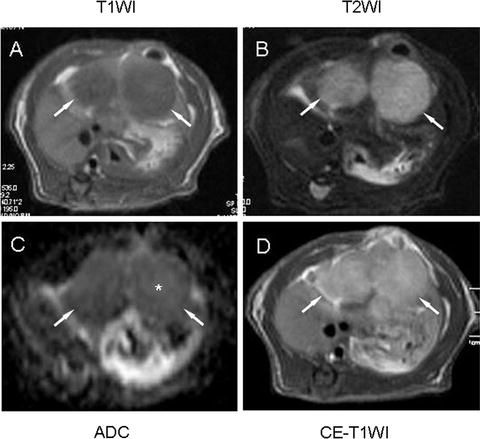
Fig. 2.

MRI visualization of rhabdomyosarcoma 16 days after implantation in a Wag/Rij rat. Two tumors (arrows) in both right and left liver lobes appear hypointense on T ₁-weighted image (T1WI) (a) and hyperintense on T ₂-weighted image (T2WI) (b). Apparent diffusion coefficient map (ADC) (c) shows slight hyperintensity in the center of tumors indicating potential necrosis (*). Contrast-enhanced T1WI (CE-T1WI) shows hyperintense tumors after i.v. injection of contrast agent (d).

Only gold members can continue reading. Log In or Register to continue