(1)
Advanced Light Microscopy Unit, Centre for Genomic Regulation, Barcelona, Spain
(2)
Imaging and Cytometry Laboratory, Technology Facility, Department of Biology, University of York, York, UK
Abstract
The ongoing progress in fluorescence labeling and in microscope instrumentation allows the generation and the imaging of complex biological samples that contain increasing numbers of fluorophores. For the correct quantitative analysis of datasets with multiple fluorescence channels, it is essential that the signals of the different fluorophores are reliably separated. Due to the width of fluorescence spectra, this cannot always be achieved using the fluorescence filters in the microscope. In such cases spectral imaging of the fluorescence data and subsequent linear unmixing allows the separation even of highly overlapping fluorophores into pure signals. In this chapter, the problems of fluorescence cross talk are defined, the concept of spectral imaging and separation by linear unmixing is described, and an overview of the microscope types suitable for spectral imaging are given.
Key words
Spectral imagingLinear unmixingImage analysisFluorescence cross talkMultichannel imaging1 Introduction
The introduction of fluorescent dyes for microscopy and their combination with immunochemistry provided important stimuli for light microscopy after decades of relative stagnation in regard to new developments. The possibility to exclusively visualize highly specific intracellular structures in distinctive colors against a dark background has changed our visual perception as well as our understanding of cellular mechanisms. The replacement of photographic film by highly sensitive monochromatic CCD cameras that generate digital images that can be easily merged into dramatic multicolor images helped to establish fluorescence light microscopy as the method of choice for cell biological imaging. Fluorescence imaging was also ideally suited for a groundbreaking new technology, confocal microscopy, which emerged as a powerful tool for biological imaging at the end of the 1980s and allowed the generation of highly resolved three-dimensional datasets of biological samples. The cloning of genes for autocatalytic fluorescent proteins in the middle of the 1990s allowed the observation of living structures in fluorescence with unprecedented ease and revolutionized the field of in vivo imaging, as acknowledged in the 2008 Nobel Prize for Chemistry awarded to O. Shimomura, M. Chalfie, and R. Tsien.
These days, the availability of an elaborate palette of fluorescent dyes extending even beyond the visible spectrum, an almost equally well-distributed range of fluorescent proteins and instruments capable of simultaneously acquiring dozens of spectral image channels provide us with an unprecedented richness in labeling possibilities [1–4]. This however also highlights inherent limitations in the specificity of fluorescence signals. Even though commonly used fluorophores seem to possess very distinct color signatures to the eye of the observer, their true spectral distributions are wide and significantly overlapping with the spectra of other fluorescent dyes. Some combinations of fluorophores, as well as a higher number of labels within one sample, will result in signals that cannot reliably be separated. Incomplete separation however makes quantitative analysis or the study of localization impossible.
Recently the analysis of spectral datasets and the signal separation by linear unmixing to overcome these problems have become widely used. Spectral imaging was initially used for spectral karyotyping [5] and subsequently combined with linear unmixing for immunohistochemistry [6]. It generated much interest after being applied to two-photon microscopy [7] and subsequently to confocal microscopy [8].
In this chapter we are going to define the problems inherent in fluorophore cross talk and cross-excitation and we are going to highlight the instrumentation and the processing methods that allow the reliable separation of multiple fluorescence signals.
2 Fluorescence Cross Talk and Cross-Excitation
Fluorescence at the molecular level consists of the ability of a molecule to absorb the energy of a photon and to subsequently reemit a photon of less energy. Only photons within a certain energy range can be absorbed and the fluorescence emission can only happen within a second defined energy range. The wavelength of a photon is inversely proportional to its energy level, so that this relation can also be described inside the color spectrum of light, with longer (i.e., “red”) wavelengths corresponding to lower energy levels. The difference between the wavelength at which a fluorophore is most efficiently excited and the wavelength at which most emission photons are generated is referred to as the Stokes’ shift. In reality fluorescence phenomena are far from monochromatic. The wavelength maxima are embedded in much wider excitation and emission spectra which represent the efficiency of excitation at a certain wavelength and for the emission side the likeliness of a photon being generated at a certain wavelength. Most fluorophores have near mirror image symmetry between their excitation and emission spectra, with the excitation spectra extending to significantly shorter wavelengths than the excitation maximum and with emission wavelengths tailing far to the red of the emission maximum (Fig. 1). Even for fluorophores with fairly defined spectra, each spectrum can cover around 100 nm, meaning that, inside our spectrum of visible light from 350 to 700 nm, most fluorophores are excitable or detectable over a significant range [9].

Fig. 1
Excitation profile (blue line) and emission profile (green line) of Fluorescein isothiocyanate (FITC) excited with a 488 nm argon laser (broken line). Stokes shift is illustrated by the double arrow. The long slopes of the excitation spectrum to the blue and of the emission spectrum to the red are clearly visible
Fluorophore cross talk can be defined as the overlap of the emission spectra of two different fluorophores. In practice it means that, depending on the spectral region chosen for detection, the signal will consist of contributions from both fluorophores if both are excited at the same time (Fig. 2). Fluorophore cross-excitation describes the phenomenon of simultaneous excitation of two fluorophores due to the fact that at the excitation maximum of one of them, the other can often be excited with significant efficiency. Sometimes, both phenomena are jointly referred to as fluorophore cross talk, but for a more thorough understanding, it is useful to separate them. Another frequently used term is bleed-through.

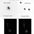
Fig. 2
(a) Excitation and emission spectra of FITC (solid lines) and propidium iodide (broken lines) showing the laser lines at 488 nm and 543 nm (black). The emission filter sets routinely used are shown below the spectra and the level of FITC emission which bleeds through into the red channel during simultaneous data collection using a 560 long pass emission filter is blocked in red. (b–g) Confocal images of a gut section labeled with anti-glucose transporter 5 and a secondary FITC antibody (green) and the nuclear stain propidium iodide (red). (b)–(d) are imaged simultaneously and (e)–(g) are imaged sequentially. FITC emission is shown in green (b, e, 488 nm excitation, 505–550 band pass emission) and propidium iodide emission is shown in red (c, f, 543 nm excitation, 560 long pass emission), (d, g) Composite images of the green and red channels. The bleed through of FITC emission into the red channel during simultaneous collection is highlighted by the arrows in (c) and consequently alters the color of the green localization in (d)
Specificity problems in samples with several fluorescence stains may be compounded by the fact that, depending on their efficiency in absorbing and also in emitting photons, some fluorophores are significantly brighter than others. Combinations of “dim” and “bright” fluorophores may cause problems in reliably identifying the signals of the “dim” dyes. The same problem can arise even if both fluorophores are equally bright, but their relative concentrations in the sample are significantly different.
Methods to insure a reliable identification of the fluorescence signals in a sample containing several labels are therefore a fundamental requirement for the analysis of fluorescence microscopy images.
Even though the wide spectra of fluorophores are indeed prone to problems of cross talk and cross-excitation, specific recognition of fluorescence microscopy signals has been successfully achieved for most standard applications. The use of properly configured fluorescence filtersets, i.e., the ensemble of excitation filter, dichroic mirror, and emission filter, achieves a reliable separation of the signals of the most commonly used fluorophore combinations. This separation is possible because the characteristics of most fluorophore spectra are the following:
Excitation spectrum: Long tail to the shorter (“blue”) wavelengths, rapid drop after the excitation maximum.
Emission spectrum: Rapid rise to the emission maximum, long tail to the longer “red” wavelengths.
In a pair of two partially overlapping fluorophores A and B (with fluorophore B having spectra more shifted to the red relative to fluorophore A), B is thus likely to get cross-excited at the excitation maximum of A. However, in the shorter wavelengths of A’s emission spectrum, there will be no contribution from B, as fluorophore B only starts emitting shortly before its own emission maximum. Fluorophore A can therefore be separated reliably from B through the use of a band-pass emission filter that collects fluorescence only from that part of A’s emission spectrum that does not overlap with B’s emission. In fluorophore B’s emission range, especially around its own emission maximum, there will be significant overlap with emission from fluorophore A. However, as fluorophore A’s excitation spectrum drops rapidly after its excitation maximum, B can be excited at its own excitation maximum without any simultaneous excitation of A. Emission overlap thus becomes irrelevant as A is not emitting and B can be imaged specifically by using an excitation band-pass filter that does not overlap with A’s excitation spectrum.
This is the most commonly used solution for the imaging of standard fluorophore combinations in fluorescence microscopy. It is robust and its main disadvantage, the incomplete collection of fluorescence emission due to the use of band-pass emission filters, can be minimized by the choice of fluorophores that are bright and that are spectrally as separated as possible.
This solution becomes less applicable under several conditions:
1.
In the presence of higher numbers of fluorophores.
2.
In the presence of fluorophores that are not matched to existing filtersets.
3.
In time-limited (and exposure-limited) situations like in vivo imaging.
Karyotyping using multicolor fluorescent in situ hybridization (FisH) probes is a good example of the first case. To reliably identify all chromosomes, a high number of fluorescence signatures are needed. Specificity for such samples was initially achieved through the use of highly restrictive filter combinations, at the cost of signal efficiency [10, 11].
The second case can be encountered when dealing with genetically encoded protein-tags. The currently available fluorescent proteins offer a wide spectral distribution [1, 2, 12], but their spectra are often not matched to existing filter combinations and due to their complex properties (brightness, pH stability, oligomerization) they can not readily be “mixed and matched” solely on their spectral properties. Viable combinations often present significant problems with fluorophore cross talk (Fig. 3).

Fig. 3
Excitation and emission spectra of two frequently combined fluorescent proteins, Enhanced Cyan Fluorescent Protein (ECFP, excitation: blue, emission: cyan) and Enhanced Yellow Fluorescent Protein (EYFP, excitation: green, emission: yellow ). The normalized spectra (a) show the significant amount of overlap of the ECFP emission with the EYFP emission. Without normalization (b) it becomes clear that EYFP is the significantly brighter fluorophore due to its higher absorption and emission efficiency. YFP can also be excited with light suitable for ECFP excitation, and can provide a significant fluorescence signal that overlaps with the second half of the ECFP emission, so that a band-pass filter is needed to insure specific detection
The use of specific filtersets for multichannel fluorescence imaging normally requires sequential acquisition of the different channels. The more channels there are to be acquired, the longer the whole acquisition process takes. During in vivo experiments, the observed process may be so fast that the next image of a time-series already needs to be taken when the acquisition of all channels is not even finished. Also, a living sample may change even while the different fluorescence channels are being recorded, so that the information in the channels is not completely matched.
Confocal microscopes generally have more than one fluorescence detection channel and therefore could be used for more time-efficient parallel acquisition of several channels. If the aim is however to separate fluorescence signals clearly into detection channels confocals can be operated in sequential imaging modes with the same problem of accumulating acquisition times. Simultaneous excitation of several dyes would immediately lead to problems with fluorophore cross talk and it is normally avoided by offering the possibility of imaging modes like “multitracking,” “sequential imaging,” etc.
The cases described above make it clear that standard fluorescence imaging approaches cannot provide solutions for some of the current experimental requirements of biological imaging.
Recent instrument developments and the implementation of image processing approaches originally established in remote sensing do however provide solutions, allowing the clear separation even of highly overlapping fluorescence signals.
3 The Concept of Spectral Imaging and Linear Unmixing
In remote sensing, multiband images taken by satellites represent the same geographical region in distinct spectral channels of the visible and also the invisible (and radar) spectrum. The signals of different types of vegetation and geological formations show a characteristic spectral distribution and are in this aspect similar to the emission spectra of fluorophores.
For the analysis of such multiband images, approaches have been developed that allow a clear assignment of distinct spectral signatures to specific ground features, even though such signatures are not specific for one image channel, but distributed over many image channels (called image bands) and significantly overlapping with one another [13, 14]. In the last years some of the analysis methods established in remote sensing for multiband data have also been applied for multichannel fluorescence microscopy datasets [7, 8].
Three approaches were tested for the analysis of fluorescence microscopy data:
Supervised classification analysis.
Primary component analysis.
Linear unmixing.
The first two methods are classification-based. Such classification approaches have been used for some time in spectral karyotyping using multicolor FisH [5] where the labeled chromosomes have only one characteristic signature. Classification techniques do however not work for colocalized fluorophore signals such as can be found in tissues or cells. It has been shown that the third method, linear unmixing, is the one best suited to analyze mixed contributions to a pixel, as would be the case for colocalizing labels [6–8].
4 Linear Unmixing
Fluorescence signals can be described as a linear mixture of contributions coming from the fluorophores present in the observed volume. The concentration of the fluorophores in the observed spot determines their contribution to the total signal. If one looks only at parts of the total signal that would correspond to different fluorescence image channels, the relative contribution of the fluorophores to a channel will vary according to the distribution of their emission spectra, even though the concentration of the fluorophore is the same for all channels.
As a linear equation the contribution of fluorophores to an image channel can be expressed in the following way:

where S represents the total detected signal for every channel λ, FluoX(λ) represents the spectral contribution of the fluorophores to every channel, and A x represents the abundances (i.e., concentrations) of the fluorophores in the measured spot.
(1)
More generally, this can be expressed as:

or

where R represents the reference emission spectra of the fluorophores [8].
(2)
(3)
If the reference spectra R for all contributing fluorophores are known, the abundances A can be calculated from the measured signal S. The process through which this can be achieved is called linear unmixing. It calculates the contribution values that most closely match the detected signals in the channels. A least square fitting approach minimizes the square difference between the calculated and measured values with the following set of differential equations:

where j represents the number of detection channels and i the number of fluorophores.
(4)
The linear equations are usually solved with the singular value decomposition (SVD) method [6, 15], so that after the calculation of the weighing matrix (A), clear representations of the separated fluorophores can be created. The separated fluorophore signals can then be displayed as distinct image channels without contributions from any other label in the sample. The intensity distribution of the signals in each position is preserved as the total signal is redistributed into the specific fluorescence channels, but not altered. It can therefore be analyzed quantitatively.
5 Requirements for the Linear Unmixing of Spectral Datasets
5.1 Reference Spectra
To be able to calculate the fluorophore contributions, linear unmixing requires knowledge of the reference spectra for the fluorophores present in the sample (Fig. 4). For maximum accuracy, such reference spectra are best taken from samples containing only the fluorophore of interest. They can also be taken from mixed samples, if specific regions only contain the signal of interest, but this contains a risk of introducing contaminating contributions from other fluorophores.

Fig. 4
 Confocal Imaging of Butterfly Tissue
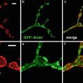 Confocal Imaging of Fluorescently Labeled Proteins in the Drosophila Larval Neuromuscular Junction
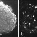 Vital Imaging of Multicellular Spheroids
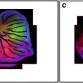
 Imaging Tools for Analysis of the Ureteric Tree in the Developing Mouse Kidney
 Evaluating Confocal Microscopy System Performance
 Laser Scanning Confocal Microscopy: History, Applications, and Related Optical Sectioning Techniques


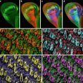
Gallery of 16 YFP emission images spanning 456–628 nm in bins of 10.7 nm of 293T cells transfected with a plasmid expressing YFP transiently throughout the cell. YFP was excited using a 514 nm laser with a HFT 458/514 main dichroic, and a Plan-Apochromat 63×/1.4 oil DIC objective. The wavelength data on each image represents the center point of each 10.7 nm bin. A spectral curve for YFP emission (b) covering the range of the wavelength scan can be generated from the proportions of YFP fluorescence in the 16 bins
Related posts:
Confocal Imaging of Butterfly Tissue
Confocal Imaging of Fluorescently Labeled Proteins in the Drosophila Larval Neuromuscular Junction
Vital Imaging of Multicellular Spheroids
Imaging Tools for Analysis of the Ureteric Tree in the Developing Mouse Kidney
Evaluating Confocal Microscopy System Performance
Laser Scanning Confocal Microscopy: History, Applications, and Related Optical Sectioning Techniques
Stay updated, free articles. Join our Telegram channel
Full access? Get Clinical Tree
