(1)
Reproductive Toxicology Division, National Health and Environmental Effects Research Laboratory, Office of Research and Development, U.S. Environmental Protection Agency, Research Triangle Park, NC, USA
Abstract
A confocal microscope was evaluated with a series of tests that measure field illumination, lens clarity, laser power, laser stability, dichroic functionality, spectral registration, axial resolution, scanning stability, PMT quality, overall machine stability, and system noise. These tests will help investigators measure various parameters on their confocal microscopes to insure that they are working correctly with the necessary resolution, sensitivity, and precision. Utilization of this proposed testing approach will help eliminate some of the subjectivity currently employed in assessing the CLSM performance.
Key words
Confocal microscopeLasersCoefficient of variationPhoto multiplier tubesField illuminationAxial resolutionSpectral registrationLaser stabilityBeadsMicroscope lensesQuality assuranceQuantificationSpectroscopy1 Introduction
The confocal laser-scanning microscope (CLSM) has enormous potential in many biological fields. When tests are made to evaluate the performance of a CLSM, the usual subjective assessment is accomplished by using a histological test slide to create a “pretty picture.” Without the use of functional tests many of the machines may be working at sub optimal performance levels delivering suboptimum performance and possibly misleading data. In order to replace the subjectivity in evaluating a confocal microscope, tests were derived or perfected that measure field illumination, lens clarity, laser power, laser stability, dichroic functionality, spectral registration, axial resolution, scanning stability, PMT quality, overall machine stability, and system noise. These tests will help serve as a guide for other investigators to ensure that their machines are working correctly to provide data that is accurate with the necessary resolution, sensitivity, and precision. Utilization of this proposed testing approach will help eliminate the subjective nature of assessing the CLSM and may allow different machines to be compared. These tests are essential if one is to make intensity measurements.
The CLSM has been evaluated by using the following biological test samples: beads, spores, pollens, diatoms, fluorescent plastic slides, fluorescence dye slides, silicone chips, and histological slides from plants or animals [1–14]. In most cases the test sample is of biological origin and is sometimes used in the course of research in the individual’s research laboratory. This is a testing procedure recommended by the manufacturers of most CLSM equipment. In the author’s opinion, this is too arbitrary a test when applications (i.e., intensity measurements or colocalization studies) other than “pretty pictures” are needed. Unfortunately this technology does not have a single universal standard by which the investigator can evaluate their CLSM. It would be advantageous to have better methods for the investigator to evaluate system performance and image quality.
The CLSM consists of a standard high end microscope with very good objectives, different lasers to excite the sample, fiber optics to deliver the laser light to the stage, acoustical transmission optical filters (AOTF) to regulate the laser light delivered to the stage, barrier filters, dichroics, pinholes to eliminate out of focus emission light, electronic scanning devices (galvanometers), detection devices to measure photons (i.e., PMTs) and various other electronic/optical components. For this system to operate correctly, it is important for it to be properly aligned and to have all the components function correctly. Instrument performance tests that have been devised include the following: laser power, laser stability, field illumination, spectral registration, lateral resolution, axial Z resolution, lens cleanliness, lens functionality, and Z-drive reproducibility [1–13]. This list is not inclusive and additional parameters may be needed to assess whether the CLSM is indeed working properly.
Since a confocal microscope can provide spectacular 3D data of biological structures, there is sometimes a tendency to overlook many of the quality assurance (QA) parameters that may be needed. The CLSM may function at sub-optimum conditions for long periods of time delivering inferior data with the problems being resolved only when the investigator cannot achieve the desired images or there is a hard failure of the equipment necessitating a service personnel visit. Sometimes inferior performance of a CLSM may be attributed to a bad sample preparation of the specimen that is imaged. However if the CLSM is not working correctly, the images and data derived from a confocal microscope may be incorrectly interpreted. Since all the CLSM images are digital and made with sophisticated optical equipment, it is now possible to derive tests that can be used to evaluate many of the machine’s components. It is the recommendation that the CLSM microscopes should not be evaluated by deriving a “pretty” image from a histological slide. QA on the CLSM is essential to insure it is performing properly and delivering accurate and reproducible data. This review attempts to incorporate QA procedures into the operation/maintenance of confocal microscopes to improve the reliability of the machines and the data quality. This review also emphasizes that scientists need to evaluate their CLSM system performance to insure that the machine is working properly. It is their responsibility to insure the machine is functional.
2 Materials
2.1 Confocal Microscope
The majority of data presented in this manuscript was derived on either a Leica TCS-SP1 (Heidelberg, Germany) confocal microscope system. This system contained an argon–krypton laser (Melles Griot, Omnichrome) emitting a 488, 568, and 647 nm lines and a Coherent Enterprise UV laser emitting 351 and 365 nm lines. The system contains an AOTF and the following three dichroics for visible light applications: single dichroic (RSP500); double dichroic (DD); and triple dichroic (TD). These tests derived on a Leica system were shown to be applicable to other point scanning systems that contain different types of lasers, objectives or other hardware configurations. For comparison purposes, similar tests were made on two different Zeiss 510 units containing three lasers [Argon 488 (25 mW); HeNe 543 (1 mW); and HeNe 633 (5 mW)] with a merge module and an AOTF. For additional comparison purposes, similar tests were made on a Leica AOBS unit that contained four lasers UV (Argon 351, 365 Enterprise) [Argon 488 (50 mW); HeNe 543 (1.2 mW); and HeNe 633 (10 mW)] with a merge module and an AOTF.
2.2 Field Illumination: Fluorescent Slides
The field illumination test slides consisted of three fluorescent plastic slides (Delta, Applied Precision Inc, Issaquah, Washington) which had excitation peak wavelengths of 408 nm (blue), 488 nm (orange), and 590 nm (red) and emission peak wavelengths of 440, 519, and 650 nm, respectively. The orange slides (488 nm) were used to test for visible field illumination and alignment. The blue slides (408 nm) were used for UV field illumination and alignment. Field illumination can also be measured using four Fluor-ref slides (Microscopy Education, Springfield, Mass) or four Chroma slides (Chroma, Brattleboro Vermont). These slides work equally well for field illumination tests. Spectral tests were made with the Red Chroma slide. They work well if the surface is clean and free of debris and it may be useful to protect the surface from possible scratches. By sealing a 1.5 cover slip (0.17 mm) with immersion oil or mounting medium (Vectasheild or Prolong) on top of the slide.
2.3 Power Meter
The power meter used to measure light on the microscope stage was a Lasermate Q (Coherent, Auburn, CA) with visible (LN36) and UV detectors (L818). A power meter (1830C) from Newport Corporation with an SL 818 visible wand detector can also be used for power measurements. A remote control box for the Coherent UV Enterprise laser was used to regulate UV laser power (0163-662-00, Coherent, Santa Clara, CA). On most confocal systems there is a 10× lens: Zeiss uses a 10× Plan Neofluar (NA 0.3) and a Leica has a 10× Plan Fluorotar (NA 0.3) or 10× Plan Apo (NA 0.4). The dry 10× lens was used to take power measurements. The machinist’s plans for building the power detector holder are available by e-mailing the author.
2.4 Beads
Various bead types and sizes are useful as test particles to access different aspects of machine functionality. It is useful to have point-spread beads (0.17 μmol Probes) and micron sized particles (0.5–1 μm sized beads, and 4–10 μm beads). The beads having different fluorescent excitation wavelengths were obtained from Spherotech (Libertyville, IL) or Molecular Probes (Eugene, OR). Other manufactures also make suitable beads.
The following Spherotech beads were used: 10-μm Rainbow (EX 365, 488, 568) fluorescent particles (FPS-10057), Yellow beads (5.5 μm FPS-5052, EX 488); UV beads (5.5 μm FPS-5040) EX 365; Blue beads (5.5 μm FPS-5070, EX 647). The 6.2-μm Rainbow beads with three different intensities (FPS-6057-3) were used for early statistical PMT tests. The following PSF Rainbow beads were used: (0.16 μm, FP-02557-2s), (0.5 μm, FP 0857–2), and (1.0 μm FP-0557-2). The polystyrene 10-μm beads (RI = 1.59) were mounted with optical cement (RI = 1.56) on a slide using a 1.5 size cover glass. The Leica immersion oil has a refractive index of 1.518.
The following Molecular Probes beads were used: Tetraspeck beads (T7282 0.5 or 1-μm) EX 365, 488, 568, 647) were used for spectral registration tests and point spread functions (PSF); PSF beads (175 nm P-7220) of different wavelengths were used for acute deconvolution PSF measurements; 15 μm focal check beads (F24634 kit) consisting of orange ring and blue throughout (F7236) for UV and visible colocalization or green, orange, and dark red ring stains (F7235) for visible colocalization of the 488, 543, and 633 laser lines.
Bead slides were made by dropping 3–5 μl of diluted beads onto a slide, allowing the liquid to dry and then covering the spot with Permount, glycerol, water, or oil and sealing it with a #1.5 cover glass. Antifade mounting media from Vector (Vectoshield H-1000) or from Molecular Probes (Slowfade light S-7461) is useful to decrease bleaching.
2.5 Biological Test Slides
FluoCells (F-14780, Molecular Probes, Eugene, OR) were stained with three fluorochomes (Mitotracker Red CMXRos, BODIPY FL phallacidin, DAPI) and used as biological test slides. Additional slides were made in our laboratory with cells grown on cover slips, fixed with Paraformaldehyde, and stained with DAPI for UV excitation or other suitable fluorochromes for visible excitation.
2.6 Axial (Z) Resolution Test
The axial resolution of the CLSM is tested using a single reflecting mirror obtained from Leica or Edmonds Scientific. A 21 mm square (#31008 Edmonds Scientific, Philadelphia, PA) was glued onto a microscope slide and a cover glass (#1.5 Fischer, Pittsburgh, PA) was placed on top of the slide with a drop of immersion oil (Leica Immersion oil, n = 1.518) The cover slip is placed firmly onto the mirror to remove all excessive oil. This type of standard test slide can also be obtained from a confocal manufacturer (Leica) or Spherotech (Libertyville, IL).
2.7 Square Sampling
It is important to ascertain whether there was square sampling or rectangular sampling in an image. A computer chip was glued onto a glass slide and used as a test substrate. A commercial product can also be obtained from MicroBrightField (Williston, VT) or Geller MicroScientific (Topsfield, MA) or Richardson Microscopic. A digital TIFF image was obtained using a dry 20× objective and the number of small boxes observed was counted by eye in the vertical and horizontal directions. If there is the same number of boxes per inch in the vertical and horizontal directions, then it can be assumed that the sampling of pixels is square. If they are not equivalent, then the sampling of pixels is rectangular, which is undesirable. This test can also be used for galvanometer stability and proper functioning.
2.8 Software Analysis
The analysis of the images was made on workstations that contained Leica, Zeiss, and Bitplane (Zurich, Switzerland) software packages. If necessary, the TIFF images were imported into Image Pro Plus (Media Cybernetics, Silver Springs MD) or Image J (NIH) for more intensive measurements and analysis. Colocalization software includes Cool Localization and Bitplane software.
2.9 PMT Spectral Evaluation
The PMT spectral response was measured over a large spectral region using an inexpensive PARRIS fluorescence calibration lamp (MIDL) consisting of a defined mixed ion gas (816025, LightForm Inc., Hillsborough, NJ)
3 Methods
3.1 Confocal Microscope Set Up
1.
Turn lasers on 15–30 min prior to use for experiments.
2.
If there is a variable power control it should be set at sufficient power to eliminate laser noise and when not in use the laser should be in “park” position.
3.
Objectives should be cleaned with Sparkle, MEOH or equivalent cleaner prior to use. They must be clean and should be checked often, especially when located in a Core facility. The objectives can be observed with the eyepiece objective, stereo microscope or with the axial resolution test (described below).
4.
Lens condenser diaphragm should be totally open.
5.
Microscope should be set up for Kohler illumination with the field diaphragm being totally open and the microscope lenses adjusted for parfocality.
3.2 Field Illumination
1.
Seal a 0.17 coverslip on the plastic slide (Chroma or Delta) with oil to eliminate potential scratching.
2.
The fluorescent slide was placed on the stage and the maximum intensity was found on the surface of the slide. Delta orange slide and the Chroma red slide yielded good excitation and spectral peaks and were thus used for visible or UV excitation. The blue slides were preferentially used for UV excitation.
3.
Measure the field illumination at a specific depth in the plastic slide, as the intensity distribution may change from the surface to the interior of the slide. The depth of focus was adjusted between 30–100 μm, dependent on the objective that was used [5× (100 μm); 10× (75 μm); 20× (50 μm); 40× (40 μm); 63× (30 μm); 100× (30 μm)]. Investigators should also be careful not to observe field illumination deep within the plastic slide samples, as it will usually yield a better field illumination pattern than regions closer to the surface due to light scattering.
4.
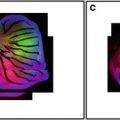
Figure 1 shows data derived from a 20× Plan Apo lens (0.7 NA) zoomed to a factor of 1.2 to illustrate a good visible field illumination (488 nm) pattern and a misaligned UV (365 nm) system yielding bad field illumination pattern. Each laser line must be checked to insure they are aligned properly as they use different dichroics to insure the beams are co localized. In addition, the field illumination of one lens is not necessary identical to the field illumination of the other lenses, necessitating that each lens be checked with the suitable dichroic that will be used in the experiment.

Fig. 1
Field illumination. Field illumination pattern of visible (a) and UV (b) excitation using a 20× (Plan Apo, NA 0.7) lens. The visible field illumination shows uniform illumination with the brightest intensity being in the center of the objective. The line running diagonally in (a) and (b) measures the histogram intensity of the field illumination graphically represented in figures (c) and (d). The variation in intensity from the left to right side of the field is less than 10 % for visible excitation and over 150 % for UV excitation. Acceptable field illumination has brightest intensity in the center of the objective decreasing less than 25 % across the field. The intensity regions were prepared by using Image Pro Plus to divide the GSV into ten equal regions and a median filter was used for additional processing. The non-uniform pattern shown in Fig. 1 with UV illumination clearly illustrates a field illumination problem, which will affect intensity measurements in an image. Although Fig. 1 was obtained with UV optics it represents the type of field illumination that can also occur with visible excitation. This pattern is unacceptable with any CLSM optical system as the maximum intensity should be in the center of the objective and not in a corner
3.3 Power Measurements
Power Meter
1.
Connect the suitable UV or visible probe (Coherent probe detectors (UV-L818, Vis-LN36) a power meter (Lasermate/Q, or Field Master, Coherent, Santa Clara, CA) and place it directly on top of the dry 10× objective. A lens holder can also be fabricated in the machine shop and placed on the stage. A different lens design, magnification, or numerical aperture (NA) will affect the laser power transmission and measurement.
The power meter is adjusted to the specific wavelength (365, 488, 568, or 647 nm) and the maximum power of laser light is read on the digital scale.
2.
The CLSM zoom factor is set from 8 to 32 to reduce the beam scan range and to focus the laser light into the “sweet spot” of the detector.
3.
The scanner is set at bi-directional-slow speed to reduce the time period that the power meter is reading “0”.
4.
The maximum digital reading from the power meter was recorded. The power derived from this measurement is dependent on the type magnification and NA of the lens used.
5.
Each lens will have a unique set of values, which is dependent on objective’s NA and other transmission factors. The power meter diode located in the machine was not reliable and could only be used as a crude relative estimate of the laser’s functioning. This internal power meter may change in the future with better-designed systems.
UV Power Test
The test was carried out in a similar manner to that described for the visible power measurement except the power meter was set for 365 nm and the UV detector (L-818) was attached to the power meter. A Coherent UV, 60-mW, Enterprise laser delivered normal power output at the laser head (over 40 mW of laser power), but only about 500-uwatt maximum power through a Plan Fluor 10× (0.3 NA). When our system had insufficient output under these conditions (approximately 500 uwatt through a 10× Leica (0.3 NA) lens) we also had insufficient light for many UV experiments using higher magnification objectives (40×, 63×, and 100×). Power throughput is a reflection of both laser status and system alignment problems
Bead or Histological Power Meter
If a power meter is not available, the crude power of the system can be also be assessed by recording the PMT voltage necessary to acquire an image at almost saturation values by using standard histological samples like the FluorCells slide (F-14780, Molecular Probes, Eugene, OR), beads like the 10-μm Spherotech beads (FPS-10057-100) or fluorescent plastic slides. The light throughput in the system can be determined by setting the laser at maximum values and recording the specific PMT voltage in which saturation of the bead occurs. If conditions are identical between machines, this PMT value can be used as a reference value to compare CLSM units and to establish their acceptable performance levels. Leica technicians routinely use a 40× lens to measure the fluorescence saturation of a histological stained plant sample (Convalaria). If the plant sample saturates in the PMT range between 600 and 700 units in PMT 1 the system is passed as having adequate power by confocal technicians.
3.4 Axial (Z) Resolution
Axial (Z) Resolution (Mirror)
The axial resolution test is considered the “gold standard” of resolution in confocal microscopy [1, 2, 5, 11, 14]. Although it is not the only criteria for a good image, the axial resolution of the system should be maximized to yield a minimal axial Z-Resolution value with a symmetrical histogram and minimal spherical smaller diffraction peaks (Fig. 2)

Fig. 2
Axial resolution. The axial resolution was made with two 63× lenses (NA 1.32) at different times on the same Leica TCS-SP1 confocal system. The peak intensity of the histogram is approximately 235 and the half-maximum intensity is at 117. One lens gave an excellent Full-Width Half-Maximum (FWHM) of 285 nm (a) while the other lens yielded a bad value of 510 nm (b). The system was aligned properly in both cases. The axial resolution of a Plan APO 63× (1.32 NA, 285 nm) showing a symmetrical major peak and a diffraction pattern consisting of smaller peaks and valleys (a). This pattern is suggestive of an excellent quality lens A. By accident, a dirty lens with dried oil was measured and it also was found to have a larger FWHM (c). However the pattern of this dirty lens showed a peak with a shoulder suggestive of spherical aberrations which is not desirable. It is important the FWHM be as low as possible and the histogram pattern look like (a) and not (c). Lens B shows a distribution with the collar partially closed which increases the FWHM. System with higher FWHM will perform less effectively. The lens with the lower FWHM is desirable for good biological resolution
1.
Place the mirror on the stage and use a high NA oil lens (63× or 100×).
2.
Set the microscope up in reflecting mode using a RT 70/30 dichroic.
3.
Fully open up lens condenser so lens is operating at highest NA.
4.
Using XY scanning mode one should find the reflected surface of the mirror keeping the pinhole aperture open for good light transmission. This will be the brightest intensity. Zoom should be 1.
5.
Switch to XZ scanning mode.
6.
Find the reflecting line and adjust it so it is located in the middle of the field.
7.
One may adjust the offset so there is a little background. This will reduce the axial value by about 7 nm but it will allow the diffraction pattern to be better observed.
8.
Adjust the Zoom to approximately10× and reduce the pinhole to minimum size values (20 μm on a Leica SP and 10 μm on a Zeiss 510).
9.
The reflected image is then obtained and the intensity histogram line profile across the image to determine the full-width half-maximum (FWHM) distance.
10.
The maximum intensity of the peak is determined and then the half-maximum intensity value of the histogram is obtained. This value is the axial resolution of the system with the specific lens.
11.
The specification for axial registration in a Leica TCS-SP system using 100× NA 1.4 is below 350 nm. A Leica 63× (NA = 1.32) has yielded values of 310 nm although a value of 400 nm is acceptable. There are no other lens specifications using a confocal microscope.
12.
The histogram data can be observed graphically or it can be transferred into Excel to measure the peak and the half-maximum values.
13.
14.
These axial registration values will change dependent on lens quality, cleanliness of the lens and system alignment. A dirty lens will yield and asymmetrical pattern (Fig. 2c) and a lens with a partially opened condenser (Fig. 2b) will yield a lower NA and thus will show a wider histogram distribution (Fig. 2b, c).
Wider histograms and higher FWHM are suggestive of a system that is not performing well due to alignment problems, lens NA or lens cleanliness.
Axial (Z) Registration (Beads)
Small beads (0.5–1.0 μm) from Molecular probes (Tetraspec, T7284) or Spherotech (Rainbow, FP–0857-2) are first located in the XY direction and then scanned in the XZ direction. The power is adjusted for saturation and then they are zoomed approximately 8× and averaged 4×. The size of the bead in the horizontal is compared to the vertical size. The difference between the two numbers will yield the axial resolution of the lens. This method is slightly more subjective than the gold standard axial resolution mirror test but it does yield similar values. For unknown reasons, the bead derived axial values may be better or worse than the mirror tests.
3.5 Square Pixels and Phase Alignment and Galvanometer Check
The pixel size and symmetry in XY directional field scanning can be checked by using a computer chip attached to a glass slide or a slide obtained from Microbright, Geller MicroScientific or Richardson scientific.
1.
The confocal should be set up in reflective mode (RT 70/30) using a 10× or 20× dry lens.
2.
The slider should be placed over the excitation line and the PMT should be adjusted.
3.
The small boxes or reticule lines in the vertical and horizontal direction should be compared by either counting them or by a measuring a standard line across them.
4.
This test insures that the scanning in the X and Y directions yields a perfect square and the information will be registered correctly. If there is the same number of boxes per inch in the vertical and horizontal directions, then it can be assumed that the sampling of pixels is a square. If they are not equivalent then the sampling of pixels will be rectangular, which is not desired.
5.
This test can be used to assure that alignment exists in bi-directional scanning.
Galvanometer Check
1.
Set the system up in reflecting mode with the PMT detector positioned over the 488 excitation line.
2.
Acquire only one scan and then observe the grid pattern ( i.e., Microbright).
3.
Acquire 25 sequential scans each separated by only a few seconds. Average the 25 scans and get a maximum projection.
4.
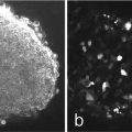
Compare the width of the grid lines with one scan and 25 scans. They should be identical but if there is a widening of these lines with the 25 scans, it suggests the system has a faulty galvanometer (Fig. 3).

Fig. 3
A MicroBrightField slide contains a rectilinear grid that can be used to detect if the field being scanned is actually square and not oblong. Using reflection mode, the detector PMT placed directly over the laser line and a grid pattern is observed. As shown in (b) (insert of partial grid) the boxes in the vertical and horizontal direction should be equivalent and straight. A malfunctioning galvanometer is shown by rectangular irregular boxes, jagged edges in the scan or irregular vertical lines. If a horizontal line is drawn over a few of the squares in (a), the width of it should be the same with one image as it is with 25 images that are sequentially acquired with a time delay of approximately 2 s between images. (a) shows a very narrow distribution which is widened after 25 sequential images are acquired. Widening of the vertical lines will indicate a badly functioning galvanometer. Tests should be run with a zoom setting of 1 and a dry 20× lens. Irregular vertical lines showing jagged edges or bends as shown in (b) will also indicate problems with the galvanometers
5.
This test can also be shown visually by comparing sequential scans. They should be identical with no widening of the lines.
3.6 Spectral Registration (Lenses and Lasers Lines Using Small Beads, Mirror, and Focal Check Beads)
Spectral Registration of Laser Lines with 1 μm Beads (UV and Visible)
The 1 μm multiple wavelength fluorescent beads (Tetraspec, T7284 Molecular Probes, or Rainbow beads, FP–0857-2 Spherotech) were used to monitor the visible spectral registration of the following lenses: (100× Plan APO, NA 1.4; 63× Plan APO, NA 1.2; 63× Plan APO, NA 1.32, Plan Fluor 40×, NA 1.0).The bead could also be used to measure the registration between multiple laser lines (UV and 568 nm).
1.
The bead was located at low zoom values in XY and the gain (slightly saturated as bleaching will occur) and offset were adjusted to their respective optimum image quality levels.
2.
An XZ scan was obtained at the proper zoom magnification (4–8×) to observe the bead. Care was made to make adjustments at the lower power levels to reduce possible bleaching effects and zoom values.
3.
By balancing laser light intensity with the Acoustical Optical Transmission Filter (AOTF), the fluorescence emission cross talk between the detection channels was minimized. If too much crossover exists the test will be invalidated. To check for cross talk, one laser light line is closed with the AOTF and the signal is observed in the other channels with the PMT voltage setting that is necessary to acquire the proper signal. It will be necessary to decrease the laser power with the AOTF and increase the PMT voltage which will help to eliminate cross talk.
4.
The bead was imaged (XY and XZ scans) with an 8–24× zoom, a slow to medium scanning rate, and frame averaged 4–8 times at two different times. The registration of fluorescence images derived from beads using the 365 nm UV laser wavelength and the 568 nm visible laser wavelength in an aligned system was almost superimposable (Fig. 4a). However at a later time, in a misaligned system, the XZ registration between the 365 nm UV line and the 568 nm visible line was not super imposable (Fig. 4b). The misaligned had a difference between the peaks of 650 nm while an acceptable difference between the two emission peaks was 210 nm. This test is critical for colocalization studies. The 568 nm line was chosen instead of the 488 line to minimize possible bead crossover fluorescence between the visible and UV wavelengths.

Fig. 4
(a, b) Spectral registration (UV and Visible). The XZ spectral colocalization of this UV (365 nm) and visible wavelength (568 nm) was evaluated with a 100× Plan Apo NA 1.4 lens using a 1 μm multiple wavelength fluorescent bead (Tetra Spec T7284 Molecular Probes). An aligned system has a full-width half-maximum (FWHM) of less than 210 nm (a) while a misaligned system has a FWHM difference of 650 nm (b). The bead was imaged using XZ scans with a 24× zoom, a slow scanning rate, and averaged eight times. The 568 line was chosen instead of the 488 line to minimize the crossover between the visible and UV wavelengths
Spectral Registration of Laser Lines with Reflective Mirror
This spectral registration test demonstrates the CLSM ability to colocalize different wavelengths of fluorescence in the same plane. To evaluate the spectral registration of the 488, 568, and 647 nm lines, a front surface, single reflective mirror (Fig. 4) was used to check visible spectral registration in a Leica TCS-SP system, in a similar manner to what was described in Fig. 2 for axial Z registration.
1.
In the Leica SP system, a 10 nm refection bandwidth is put over each excitation wavelength and the reflection can be measured sequentially with one PMT or simultaneously with three PMTs. This is similar to axial resolution test using reflection mode and XZ scanning which can be acquired sequentially or simultaneously for the three laser lines.
2.
By tweaking the AOTF and PMT voltage adjustments, the reflected light is adjusted so the maximum peak is close to 255 but does not exceed it. The intensity of each reflected line was adjusted for a maximum intensity of the image was approximately 250 GSV.
3.
The images representing three laser lines (i.e., 488, 568, 647) are displayed as an overlay and a line is drawn through the composite image. The overlapping histograms will represent three laser lines and will have a distribution representing the spectral registration of optical system with an argon–krypton laser to distribution represents the lens quality (Fig. 5).

Fig. 5
Lens spectral registration (visible). The visible spectral registration of a 100× Plan Apo NA 1.4 objective was evaluated using a front surface, single reflection mirror with the same lens at different times. A 10 nm slit is put over each wavelength and the reflection of each line was measured sequentially. The AOTF and PMT intensity was adjusted so the maximum intensity of each line was 250 GSV. Lens B was sent back to the factory, as it did not meet the following: (1) spectral registration for UV (365) and visible (568); (2) spectral registration for the three visible lines; and (3) axial resolution specifications. The refurbished Lens A showed excellent registration between the three visible lines with the difference being less than 220 μm. Refurbished Lens A also had an axial registration below 350 nm. This single reflection mirror test will yield slightly better spectral registration than 1 μm bead data for the 647-excitation line, as the fluorescence emission occurs in the far-red range (>660 nm) and many lenses have difficulty colocalizing this far red emitted light with the fluorescence emitted from the 488 and 568 wavelength excitation
4.
With the multilaser system the distribution represents the composite of lens spectral properties and the laser alignment. Studying multiple magnification lenses should allow one to determine if lens quality or system alignment is correct.
Spectral Registration of Laser Lines with Beads
1.
A 1-μm bead can be used to test visible wavelengths for colocalization in a similar manner to that described for colocalizing UV and visible light. Using the bead test, it is necessary to reduce the laser light to reduce bead bleaching and then adjust the laser light with the AOTF and PMT voltage so fluorescence cross talk between the different laser lines emitted wavelengths is minimized. It is also useful to suspend the beads in antifade to reduce bleaching for this test, as they will be zoomed at high magnification, which increases bleaching (Fig. 4).
Spectral Registration of Laser Lines with Focal Check Beads (UV and Visible Lines)
Molecular Probes produces a series of beads (Focal Check) that can be used to assess the different visible wavelengths from multiple lasers in a confocal system. These beads have different fluorescent excitation rings and core colors that can be used to assess colocalization of laser light from multiple lasers.
1.
To examine the UV (365) and visible lines (568) in a Leica TCS-SP1 confocal system that had an argon–krypton laser emitting three lines and a UV Enterprise laser. A 15-μm bead with UV blue interior and orange fluorescence ring exterior (F7236, Molecular Probes) was used to show that the UV and 568 lines were aligned (Fig. 4). In a similar manner, the F7237 bead consists of a UV blue core and a green ring and this can be used to show colocalization of the 488 and 365 laser lines. This bead may have slightly more cross talk than the blue core with a red ring (F7236). The laser power and AOTF should be adjusted to reduce cross talk between the emitted fluorescence. Any deviation between the concentric localization of the rings or the maximum diameter of the rings and core bead size suggests misalignment.
2.
In the newer confocal systems that have three lasers and a merge module, it is recommended to test for colocalization with focal check beads (F7235) that has three rings representing green, orange, and red or a focal check bead (F7239) that has a red ring and a green core. This test is similar to that described above for UV and 568 excitation with the F7236 bead. Using three separate visible laser excitation the bead should reveal concentric fluorescent rings that have maximum values in the same focal plane with either a XY or XZ scan. Variations will indicate a system out of alignment and lacking colocalization.
3.
Individual pinholes in a Zeiss system may have to be realigned monthly. This test can indicate if the pinhole needs adjustments and if the system is meeting the colocalization test.
4.
Smaller focal check beads should yield more accuracy.
3.7 Lens Spectral Registration
Different lenses were tested by the axial resolution single reflective mirror test described above. Figure 5 represents a 100× lens measured over a time period of approximately 6 months on the same CLSM system. On testing Lens B problems in axial resolution and spectral registration existed. The separation between the 488 and 647 nm line was 305 nm in lens B and the axial registration was 410 nm (Acceptable was 350 nm). This lens (B) was returned to the factory to correct this spectral registration problem in visible, and a spectral registration problem between UV and visible. After factory repair, lens A showed perfect colocalization between the 488 and 647 nm lines and acceptable registration between the 488, 647, and 568 lines. The UV and 568 nm (Fig. 5a) also showed acceptable registration after repair.
Depending on the laser configuration, this test can be revealing characteristic of the lens spectral registration or system alignment. In an argon–krypton laser system since all three lines are derived simultaneously, the test will reveal the lens characteristics. If a three laser system with a merge module is used it will reveal the combination of both lens characteristics and laser alignment. It is useful to make this test with more than one objective, as it will be rare that a system will contain multiple lenses with axial and spectral registration problems
3.8 Dichroic Functionality
The dichroics reflect good light and eliminate unwanted light. It is important that the most light be reflected to allow the system to operate efficiently.
1.
An API fluorescent plastic slide (orange) or Chroma Red slide was placed on the stage using either 488 or 568 excitation light. After the dichroic was switched into position, the PMT was kept constant and the mean GSV (Gray Scale Value) of a region of interest (ROI) in the image was determined for each acquisition condition. The values for the three dichroics can be compared to determine which one has the highest reflectivity (Table 2).
2.
The maximum values are normalized to 1 and the other values are reported as a percentage of the maximum GSV. It is important to use a bandpass or barrier filter to collect the desired light. Light at different regions of the spectra may have unique information and it is sometimes advisable to use a narrower bandpass with higher reflection to get the desired fluorescent information.
3.9 Laser Stability
Laser Stability (Visible, Long-Term Hours)
Laser stability measurements were made over hours to evaluate the possible fluctuations in power [1, 2, 5, 14]. The laser power fluctuations were initially measured both in PMT 1 (blue light sensitive, low noise, R6857) and in the transmission detector using a fluorescent plastic slide with very low laser power that was reduced with either neutral density filters or with the AOTF adjustments. The transmission optical system without a slide showed similar results to PMT 1 with fluorescent plastic slides and this was the desired optical system to perform this test if it exists on the system as it eliminated any possibility of bleaching, laser interaction with the substrate, and possible stage drift. Fluorescent colored slides, reflecting mirrors and beads have been used to demonstrate power stability but they are not as reliable as the transmission detector to evaluate power stability problems.
1.
To measure laser stability using the transmission optical system, the microscope is first aligned for Kohler illumination using a histological slide, which is then removed from the optical path.
2.
The laser power is adjusted by a combination of laser power and AOTF adjustment of the laser line power. It is desirable to adjust the AOTF so the transmission detector voltage remains constant for all three wavelengths. Adjust the AOTF for 647(or 633) first and then 568 (or 543) and finally 488.
3.
The image intensity is measured using the one transmission detector for the three wavelengths of the argon–krypton laser by sequentially measuring the laser light with the 488, 568, and 647 wavelengths. The test can be made with a three laser system substituting either the 543 or 561 laser lines or the 633 laser line for the 568 and 647, respectively. Only two lines are shown in Fig. 6 for clarity.

Fig. 6
(a) Laser power fluctuations. The periodic change in laser power was measured using transmitted interference optics without a slide in the optical path. The two lines show a visible system delivering 488 and 568 power fluctuations. The 488 and 568 lines are cycling periodically. These variations in this power intensity occur over hours and never seem to stabilize. To measure laser stability over time the PMT was kept constant and the laser power of the three lines was adjusted with the AOTF (only two laser lines are shown for clarity). Next, over 200 measurements were sequentially acquired every 30 s. After the test was complete, the intensity of a large ROI was evaluated and plotted over time. The laser power instability may be due to either laser light entering a fiber with an incorrect laser polarization, thermal instability in the AOTF or a badly aligned system. The reason for the source of power instability is not known. It can vary from as little as 10 % to as high as 400 %. (b) Laser power fluctuations. A red fluorescent Chroma slide was placed on the stage and it was sequentially excited with the 365(UV) and 568 laser lines. Two hundred acquisitions were made every minute for 3.3 h using a bandpass of 500–650 nm for emission. To reduce possible bleaching the laser power was reduced to minimum values using neural density filters (UV) and the AOTF (568 line). The red Chroma slide has the possibility of bleaching and possible stage drift. The data shows a “cold” system showing poser foliations. These fluctuations in visible continued after the system was warm while the UV system became very stable. The contrast between the two lines suggests that the AOTF may be introducing errors
4.
The test usually takes a few hundred scans separated by 10–30 s over a period of 2 h.
5.
The intensity of the same large ROI of the three fields is averaged and plotted over time for the three wavelengths. The goal of this test is to have a straight line with no variations in power to insure accuracy in the intensity measurements. It is not necessary to save the images in the scan but it is useful to save the data measurements in an Excel file, text file, or equivalent.
6.
Illustration of laser power: The type of laser power stability data that can be achieved with this test is represented in Fig. 6a, b. There is periodic noise in the laser system that exceeds both the manufactures (Ominichrome) laser stability fluctuations specifications of less that 0.5 % over a 2-h time period. The 488 and 568 lines have a periodic cycle and stability are never achieved (Fig. 6a). This is not a typical pattern as expected for argon –krypton laser and indicates there is instability in the system, which will affect intensity measurements.
7.
A Chroma red slide is placed in the light path and images are taken sequentially for 3 h at an interval of 30–60 s (Fig. 6b). Care is taken to reduce the laser power by the AOTF and the neutral density filters to reduce possible bleaching of the slide. Figure 6b shows wide fluctuations with the 568 visible line while the UV is relatively stable. The source of noise has not been indentified, but it is believed to be derived from the AOTF, as the light entering the AOTF has less than 1 % power fluctuations while after the AOTF the fluctuations are over 10 % and in this case the peak-to-peak variation is 400 % (40–160 GSV). The goal of this test is to achieve a flat stable line as illustrated with the UV light. Proper heat dissipation may also be attributed to laser instability.
Laser Stability (UV, Long Term)
The Coherent Enterprise laser delivers less than 1 % peak-to-peak noise and is considered very quiet and stable laser. The Coherent laser was tested in a similar manner to that described for visible lasers using the transmitted optical system or the PMT system with blue colored fluorescent plastic slides and very low laser power. A relatively stable line showing minimal fluctuations should be obtained (Fig. 7a) The temperature of the cooling system must be regulated properly or power fluctuations will occur (Fig. 7b, c). One source of power stability appears to be the way laser is cooled and how the laser heat is dissipated. This was illustrated with our Coherent Enterprise UV laser that was connected to a Coherent LP 20 water–water exchange cooler. This cooler should be set at least 10 °C above the circulating cooling water of the building and it should be set above the ambient temperature of the room. Improper set points for the LP 20 cooler resulted in temperature regulation problems of the circulating cooling water in the laser which in turn resulted in the improper regulation of the laser power (Fig. 7b).

Fig. 7
Laser stability of a coherent enterprise UV laser. The Coherent Enterprise UV laser delivers less than 1 % peak-to-peak noise. The laser was connected to an LP 20 water–water cooler, which should be set at least 10 °C above the cooling water of the building. It should also be set above the ambient temperature of the room. Improper set points for laser cooling resulted in bad thermal regulation of the laser B. Improper fiber alignment resulted in additional laser intensity variations C. The elimination of the temperature and polarization issues resulted in proper laser stability (A, 3 % power variation over time) The test was conducted by measuring the laser power stability in PMT 1 using a fluorescent plastic slide. Neutral density filters were used to reduce the power and thus minimize slide bleaching. The transmission detector optics gave similar results to the UV fluorescent plastic slide and was also used to measure UV laser stability
Fiber Optic Stability and Polarization
The fiber optics may influence artifacts due to deterioration with time or improper polarization alignment. Fiber optical problems will attenuate the laser power and necessitate using higher laser power or higher PMT settings in the operation of the CLSM.
1.
One test procedure recommended by one manufacturer to insure that polarization is correct after the alignment procedures is to wiggle the fiber optic and see if the image returns to the same intensity values suggesting the polarization are correct. This is a fairly crude test, but it will demonstrate whether the system fiber optic needs further polarization alignment. Better procedures are being tested by the manufactures to eliminate this polarization alignment problem.
2.
 Confocal Imaging of Butterfly Tissue
 Confocal Imaging of Fluorescently Labeled Proteins in the Drosophila Larval Neuromuscular Junction
 Vital Imaging of Multicellular Spheroids
 Imaging Tools for Analysis of the Ureteric Tree in the Developing Mouse Kidney
 Measurement in the Confocal Microscope
 Laser Scanning Confocal Microscopy: History, Applications, and Related Optical Sectioning Techniques


Laser stability tests over time may be related to laser polarization and fiber optics problems.
Related posts:
Confocal Imaging of Butterfly Tissue
Confocal Imaging of Fluorescently Labeled Proteins in the Drosophila Larval Neuromuscular Junction
Vital Imaging of Multicellular Spheroids
Imaging Tools for Analysis of the Ureteric Tree in the Developing Mouse Kidney
Measurement in the Confocal Microscope
Laser Scanning Confocal Microscopy: History, Applications, and Related Optical Sectioning Techniques
Stay updated, free articles. Join our Telegram channel
Full access? Get Clinical Tree
