Laser Scanning Confocal Microscopy: History, Applications, and Related Optical Sectioning Techniques

and Kevin W. Eliceiri²

(1)

Howard Hughes Medical Institute, Department of Molecular Biology, University of Wisconsin, Madison, WI, USA

(2)

Laboratory for Optical and Computational Instrumentation and Laboratory of Molecular Biology, University of Wisconsin, Madison, WI, USA

Abstract

Confocal microscopy is an established light microscopical technique for imaging fluorescently labeled specimens with significant three-dimensional structure. Applications of confocal microscopy in the biomedical sciences include the imaging of the spatial distribution of macromolecules in either fixed or living cells, the automated collection of 3D data, the imaging of multiple labeled specimens and the measurement of physiological events in living cells. The laser scanning confocal microscope continues to be chosen for most routine work although a number of instruments have been developed for more specific applications. Significant improvements have been made to all areas of the confocal approach, not only to the instruments themselves, but also to the protocols of specimen preparation, to the analysis, the display, the reproduction, sharing and management of confocal images using bioinformatics techniques.

Key words

ConfocalOptical sectionResolutionLaserFluorescenceIlluminationMicroscopyLivingFixedDigital imageInformatics

1 Introduction

The major application of confocal microscopy in the biomedical sciences is for imaging fixed or living tissues that have usually been labeled with one or more fluorescent probes. When these samples are imaged using a conventional light microscope, the fluorescence in the specimen away from the region of interest interferes with the resolution of structures in focus, especially for those specimens that are thicker than 2 μm.

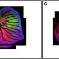
When compared with the conventional wide field light microscope, the confocal microscope provides an increase in both maximum lateral resolution (0.5 μm vs. 0.25 μm) and maximum axial resolution (1.6 μm vs. 0.7 μm). However, it is the ability of the instrument to eliminate the “out-of-focus” brightness from images collected from thick fluorescently labeled specimens at a range of magnifications that has made it an invaluable instrument for most applications in biomedical imaging (Fig. 1).

Fig. 1

Examples of Single Optical Sections from the same Specimen. Optical sections can be collected using different objective lenses or using the same lens in combination with the optical zoom function of the LSCM. In this example a fifth instar butterfly wing imaginal disk has been fixed and labeled with distalless antibodies and secondary fluorescein-labeled antibodies, and imaged in the LSCM. A single optical section of the entire imaginal disk is imaged using a 4× lens (a), whereas a 16× lens is used for improved resolution of an eyespot field (b). A 40× lens is required for cellular resolution (in this case resolution of nuclei since distaless is a transcription factor) (c). Improved nuclear resolution is achieved by using the optical zoom (d–f ) in conjunction with the 40× objective lens. This strategy is often useful when imaging at high magnifications when switching to a higher power lens will risk losing the field of interest or damaging the specimen

The method of image formation in a confocal microscope is fundamentally different from that in a conventional wide field epifluorescence microscope where the entire specimen is bathed in light from a mercury or xenon source. In contrast, the illumination in a confocal microscope is achieved by scanning one or more focused beams of light, usually from a laser, across the specimen. Images produced by scanning the specimen in this way are called optical sections [1]. This refers to the noninvasive method of image construction by the instrument, which uses light, rather than a physical method such as a microtome, to section the specimen.

The popularity of the confocal microscope has increased dramatically over the past ten years since the publication of the first edition of this book [2]. This is due in part to the increased number of confocal applications and increased accessibility of the technology and specifically to the introduction of fluorescence reporter techniques that have simplified the imaging of living cells [3].

Confocal technology has been developed to a level where most research institutions and many individual laboratories house one or more confocal instruments. In addition, instruments that produce optical sections for more specific applications continue to be developed as modifications of the confocal design [4, 5]. While the second edition, like the first, is focused on the laser scanning confocal microscope, many of the featured protocols are suitable for use with these new methods of optical sectioning [6, 7].

2 History of Confocal Instrumentation

2.1 Marvin Minsky’s Microscope

The development of confocal microscopes was, and continues to be, driven by the desire to image biological events as they occur in vivo. The invention of the confocal microscope is attributed to Marvin Minsky who built a working scanning optical microscope in 1955 with the goal of imaging neural networks in unstained preparations of living brains. Details of Minsky’s microscope, and of its development, can be found in his memoir, “On inventing the confocal scanning microscope” [8]. All modern confocal microscopes, by definition, employ the principle of confocal imaging that he patented in 1957 [9], although the term confocal was not introduced in this context until later [10].

In Minsky’s original confocal microscope the point source of light is produced by a pinhole placed in front of a zirconium arc source. The point of light is focused by an objective lens into the specimen, and light that passes through it, is focused by a second objective lens at a second pinhole, which has the same focus as the first pinhole. i.e., it is confocal with it. Any light that passes through the second pinhole strikes a low noise photomultiplier, which produces a signal that is directly proportional to the brightness of the light passing through the pinhole. The second pinhole prevents light from above or below the plane of focus from striking the photomultiplier (Fig. 2).

Fig. 2

Schematic of Marvin Minsky’s confocal microscope—transmitted light version. A point of light is produced by a zirconium light source (a) and a pinhole placed in front of it (b). This is focused by an objective lens (c) into the specimen (d), and light that passes through it, is focused by a second objective lens (e) at a second pinhole (f), which has the same focus as the first pinhole, i.e., it is confocal with it. Any light that passes through the second pinhole strikes a detector (g), which produces a signal that is proportional to the brightness of the light passing through the pinhole. The second pinhole prevents light from above or below the plane of focus from striking the photomultiplier. The image is built up by moving the specimen (d) Image drawn by Leanne Olds

The key to the confocal approach is the elimination of out-of-focus light (sometimes called flare) by scanning a point source of light across the specimen and using a pinhole to eliminate the out-of-focus light from the detector. Minsky also described a reflected light version of the microscope that used a single objective lens and a dichromatic mirror arrangement (Fig. 3). This arrangement eliminated the considerable problem of aligning the two objective lenses in the transmitted light version since a single objective lens is used for both the excitation and the emission paths. This epi-illuminated design is the basic configuration of most modern confocal systems that are used for fluorescence imaging today.

Fig. 3

Schematic of Marvin Minsky’s confocal microscope—reflected light version. A zirconium light source (a) and a pinhole (b) produces a point source of light (a). This is reflected by a dichromatic mirror (c) and focused by an objective lens (d) onto the specimen (e). Longer wavelength light is reflected back from the specimen, is subsequently focused by the same objective lens (d), passes through the dichromatic mirror (c), and focused onto a second pinhole (f) in front of the photodetector (g). Both source and detector pinholes are confocal with the focused point of light in the specimen. The image is built by moving the specimen (e). Image drawn by Leanne Olds

In order to build an image, the focused spot of light must be scanned across the specimen in some way. In Minsky’s original microscope the beam was stationary and the specimen itself was moved on a vibrating stage. This optical arrangement has the advantage of always scanning on the optical axis, which can eliminate any lens defects. However, for biological specimens, movement of the specimen can cause them to wobble, which results in a loss of resolution in the final image.

Finally an image of the specimen has to be recorded. A real image is not formed in Minsky’s original microscope but rather the output from the photodetector is translated into an image of the region-of-interest. In Minsky’s original design the image was built up on the screen of a military surplus oscilloscope with no facility for hard copy. Minsky admitted that the quality of the final images collected from his microscope was not very impressive. This was most likely due to the inferior quality of the oscilloscope display and sensitivity of the photodetector and not by the lack of resolution achieved with the microscope itself.

The images produced by Minsky’s instrument at this time were unremarkable. It is clear that the technology was not available to him in 1955 to fully demonstrate the potential of the confocal approach to the biomedical imaging community. This may have been why confocal microscopy did not immediately catch on. After all, at this time, biologists were used to viewing and photographing their brightly stained and colorful histological tissue sections using light microscopes with excellent optics, and in real color. Confocal imaging of living tissues would have to wait.

2.2 Subsequent Technological Innovation

Several major technological advances that would have benefited Minsky’s confocal design have become available to biologists during the years since 1955. These include;

Bright and stable laser light sources.

Efficiently reflecting mirrors and more precise filters.

Improved methods of scanning and electronics for data capture.

High quantum efficiency low noise photodetectors.

Improved methods of specimen preparation.

Fast computers with image processing capabilities.

Elegant software solutions for analyzing the images.

High-resolution digital displays and color printers.

Bioinformatics methods for managing the images.

The introduction of practical confocal microscopes was largely dependent upon the development of efficient methods of scanning the excitation spot within the specimen. Confocal microscopes are typically classified using the method by which the specimens are scanned. Minsky’s original design was a stage scanning system driven by a tuning fork arrangement that was rather slow to build an image. It was also extremely difficult to locate a region of interest in the specimen, and even harder to focus, using this system.

The stage scanning confocal microscopes have evolved into instruments that are used traditionally in materials science applications such as the microchip industry. Systems based upon this principle have also been used for screening DNA sequences on microchip arrays.

An alternative to moving the specimen (stage scanning) is to scan the beam across a stationary specimen (beam scanning). This configuration is more practical for imaging biological specimens, and is the basis of those systems that have developed into the current generation of research microscopes.

More details of the technical aspects of confocal microscopes are covered elsewhere [11], but briefly there are two fundamentally different methods of beam scanning; single beam scanning or multiple beam scanning. Single beam scanning continues to be the most commonly used method at this time, and is epitomized by the laser scanning confocal microscope (LSCM). Here the scanning is achieved using computer-controlled galvanometer-driven mirrors to direct a single beam of excitation light across the sample.

The alternative to single beam scanning is to scan the specimen with multiple beams (almost real time). Point-scanning LSCM, when used with high numerical aperture lenses, has an inherent speed limitation in fluorescence. This arises because of a limitation in the amount of light that can be obtained from the small volume of fluorophore contained within the focus of the scanned beam. This can be overcome with parallel or multiple laser excitation approaches. This is most commonly achieved using some form of spinning Nipkow disk; a design adapted from the early days of television transmission. The forerunner of the spinning disk systems was the tandem-scanning microscope (TSM), and subsequent improvements to the design have resulted in instruments that collect acceptable images from fluorescently labeled living specimens. The modern Nipkow or other spinning disk based variants have a much higher speed potential than conventional LSCMs because the spinning disk based parallelism avoids fluorophore saturation enabling higher levels of excitation to be used. As these systems typically optically reconstruct the image, this allows the use of high sensitivity CCD detectors giving extended red response of great advantage for many of the newly developed fluorophores. Spinning disk based confocal systems have been very popular for applications where close to real time capture is needed such as tracking calcium ion transients in cell environments.

In modern confocal microscopes the image is either built up from the output of a photomultiplier tube or captured using a CCD camera, directly processed in a computer imaging system and then displayed on a high resolution video monitor, and recorded on modern hard copy devices, with spectacular results. Moreover, vastly improved methods of specimen preparation, especially using fluorescent reporters of gene activity, have enabled the realization of Minsky’s dream of imaging living neurons in vivo.

2.3 The Laser Scanning Confocal Microscope

The LSCM continues to be the instrument of choice for most routine biomedical research applications, and it is, therefore, most likely to be the instrument first encountered by the novice user. As in the first edition, emphasis has been placed on the LSCM in this edition.

The LSCM is built around a conventional epifluorescence light microscope either in an upright configuration popular with neuroscientists and physiologists or an inverted configuration seen commonly for cell culture and developmental biology applications (Fig. 4).

Fig. 4

The main components of a modern laser scanning confocal microscope- reflected light, upright version. Light from one or more lasers passes through a pinhole, attenuated through an AOTF, bounces off a dichromatic mirror, and passes into the scanning unit. A scanned beam enters the back focal plane of the objective lens, which focuses the light at a point in the specimen. Any light coming back from the excitation of a fluorochrome at this point inside the specimen passes back through the objective lens and the scanning unit. Since this light is of longer wavelength than the excitation light, it passes through the dichromatic mirror, is further cleaned up by a barrier filter and it is eventually focused at the second pinhole. Any light that passes through the pinhole strikes a low noise photomultiplier detector, the signal from which subsequently passes to the computer imaging system of the confocal microscope. This configuration is very similar to that of Minsky’s reflected light schematic of Fig. 3. Image drawn by Leanne Olds

The conventional light microscope is essential for efficiently finding the region of interest in the specimen by eye before scanning in the confocal mode. This is extremely useful since one of the great strengths of the confocal microscope, i.e., the elimination of out-of-focus information, can make it extremely difficult to locate a region of interest in the specimen in the confocal mode. This configuration is also very stable, especially when mounted on an anti-vibration air table. Any vibration results in a loss of resolution in the image, and can show up in the image as irregular horizontal lines.

The modern LSCM typically uses a laser rather than a lamp for a light source, acousto-optic tunable filters (AOTFs) for selecting specific excitation wavelengths, dichroics for multichannel emission discrimination, sensitive photomultiplier tube detectors (PMTs) and a computer to control the scanning mirrors and to facilitate the collection and display of the images. Modern LSCMs can excite and detect multiple fluorophores simultaneously typically through the use of multiple lasers and multiple detectors for each channel. Images are subsequently stored as digital image files and can be further analyzed using additional software.

In the LSCM, illumination and detection are confined to a single, diffraction-limited, point in the specimen. This point is focused by an objective lens, and scanned across it using some form of scanning device. Points of light from the specimen are detected by a photomultiplier behind a pinhole, and the output from this is built into an image by the computer. Specimens are usually labeled with one or more fluorescent probes (fluorescence mode). Unstained specimens can be viewed using the light reflected back from the specimen (reflected light mode).

One of the more commercially successful LSCMs was designed in the late 1980’s at the Medical Research Council laboratories in Cambridge, England by the team of White, Amos, Durbin and Fordham. They set out to tackle a fundamental problem in developmental biology; namely imaging specific macromolecules in fluorescently labeled embryos [12, 13]. They were specifically interested in imaging microtubules in C. elegans embryos. Many of the cells inside developing embryos are impossible to image after the two-cell stage using conventional epifluorescence microscopy because as cell numbers rise, the overall volume of the embryo remains approximately the same, which means that the fluorescence signal increases from the more and more closely packed cells out of the focal plane of interest, and interferes with resolution of those structures in the focal plane of interest.

When he investigated the live cell imaging microscopes available to him in the mid-1980s including early confocal designs, John White discovered that no system existed that would solve his resolution issues caused by the increased signal brightness from the increased cell packing as the embryos developed over time. Technology at this time consisted of the stage scanning instruments, which tended to be impossible to focus and painfully slow to produce images (approximately 10 s for one full frame image that was often out-of-focus), and the multiple beam microscopes, which were difficult to align and the fluorescence images were extremely dim, if not invisible without extremely long exposure times!

The Cambridge team led by John White and Brad Amos designed a LSCM that was suitable for conventional epifluorescence microscopy applications and since evolved into an instrument that has been used in many different biomedical applications over the years [14]. The breakthrough came with the development of more efficient methods of scanning the beam using first a single galvanometer-driven mirror and a spinning polygon mirror design, and subsequently settling upon a dual galvanometer-driven mirror arrangement. It was also necessary to incorporate relatively new computer-based imaging technology and control electronics using a framestore card and analog to digital conversion to coordinate and keep track of the position of the scanning mirrors with the acquisition of the images into the computer. This required the development of software that was reliable and easy to use.

In a landmark paper that captured the attention of the cell biology community because of the vastly improved quality and resolution of the images of a diverse range of familiar specimens, White et al. compared images collected from the same specimens using conventional wide field epifluorescence microscopy and using their LSCM [15]. Rather than physically cutting sections of multicellular embryos their LSCM produced “optical sections” that were thin enough to resolve structures of interest and were free of much of the out-of-focus fluorescence that previously contaminated their images. This technological advance allowed them to follow and record changes in the cytoskeleton in the increasing numbers of cells in early embryos at a higher resolution than using conventional epifluorescence microscopy.

The thickness of the optical section could be adjusted simply by changing the diameter of a pinhole in front of the photodetector. The image could be zoomed with no loss of resolution simply by decreasing the region of the specimen that was scanned by the mirrors simply by placing the scanned information into the same number of pixels in the image. This imparted a range of magnifications to a single objective lens, and was extremely useful when imaging rare events when changing a lens may have risked losing the region of interest during the experiment (Fig. 1).

This design has proven to be extremely flexible for imaging biological structures as compared with some of the other designs that employed fixed diameter pinholes. This microscope together with several other instruments introduced by others during the same time period, were the forerunners of the sophisticated instruments that are now available to biomedical researchers from several commercial vendors.

The advantage of the LSCM lies within its versatility and large number of applications combined with its relative user-friendliness for producing extremely high quality images from specimens prepared for the light microscope. The first generation LSCMs were tremendously wasteful of photons in comparison to the new microscopes. This meant that photobleaching and photodamage to specimens were often problematic in the older instruments. The early systems tended to work well for brightly labeled and fixed specimens but tended to quickly kill many living specimens unless extreme care was taken to preserve the viability of specimens on the stage of the microscope by limiting the laser power for imaging. Nevertheless the microscopes produced such excellent images of fixed and fluorescently labeled specimens that confocal microscopy was fully embraced by the biological imagers.

Improvements have been, and continue to be, made to all parts of the imaging process. These include more stable lasers, more efficient mirrors, more sensitive photodetectors, electronic filters (AOTFs), improved methods for multichannel collection such as spectral based capture, and improved digital imaging systems. The new instruments have been improved ergonomically so that alignment is much easier to achieve and preserve. Filter combinations are now controlled by software and AOTFs and multiple fluorochromes can be imaged simultaneously with instrumentation for correcting for bleed through and autofluorescence (Fig. 5).

Fig. 5

The information flow in a generic laser scanning confocal microscope. Light from one or more lasers (a) passes through a neutral density filter or AOTF (b) and an exciter filter or AOTF (c) on its way to the scanning unit (d). The scanning unit produces a scanned beam at the back focal plane of the objective lens (e), which focuses the light at the specimen (f). The specimen is scanned in the X and the Y in a raster pattern and in the Z direction by fine focusing (arrows ). Any fluorescence from the specimen passes back through the objective lens and the scanning unit and is directed via dichromatic mirrors (g) to three pinholes (h). The pinholes act as spatial filters to block any light from above or below the plane of focus in the specimen. The point of light in the specimen is confocal with the pinhole aperture. This means that only distinct regions of the specimen are sampled. Light that passes through the pinholes strikes the PMT detectors (i) and the signal from the PMT is built into an image in the computer ( j). The image is displayed on the computer screen often as three grayscale images together with a merged color image of the three-grayscale images. The computer synchronizes (n) the scanning mirrors (d) with the buildup of the image in the computer frame store or memory (k). The computer also controls a variety of peripheral devices. For example, the computer controls and correlates movement of a stepper motor connected to the fine focus of the microscope with image acquisition in order to produce a Z-series. Furthermore the computer controls the area of the specimen to be scanned by the scanning unit so that zooming is easily achieved by scanning a smaller region of the specimen. In this way, a range of magnifications is imparted to a single objective lens so that the specimen does not have to be moved when changing magnification. Images are written to the hard disk of the computer or exported to various devices for viewing, hard copy production or archiving (o). Final images are produced in the computer by synchronizing input from the scan head with the video card (m). Image drawn by Leanne Olds

The development and commercial availability of fluorescent probes with improved levels of photostability and specificity for improved localization continues to influence the development of confocal instrumentation. The fluorophores include synthetic fluorochromes, for example, the Alexa dyes and quantum dots and naturally occurring fluorescent proteins, for example the green fluorescent protein (GFP) and its derivatives, for example CFP and YFP. Many of the new fluorescent probes have been designed to have their excitation and emission spectra closely matched to the wavelengths delivered by the lasers supplied with most commercial LSCMs (Table 1). The instruments continue to be improved as new technologies from diverse sources are added to the existing LSCM designs.

Table 1

Peak excitation and emission wavelengths of some commonly used fluorophores

Alexa Fluors	350 thru 680	442 thru 702	He–cadmium
Cyanines	489 thru 710	506 thru 805	He–cadmium
DAPI	350	470	He–cadmium
Fluorescein	496	518	Argon ion
GFP	395/475	510	Blue diode
Qdot	350 thru 600	525 thru 655	Blue diode
Rhodamine B	540	625	Green He–Ne
DsRed	558	583	Green He–Ne
X-Rhodamine	580	605	Krypton–argon
TOTO3	642	661	Krypton–argon

3 Confocal Imaging Modes

The value of the LSCM for biomedical imaging is due to the ability of the instrument to both scan and detect a point of light under extremely fine control in the X, the Y and the Z direction within a fluorescently labeled specimen at various time and wavelength resolutions. The basic imaging modes of the instrument will be described.

3.1 Single Optical Sections

The basic output of all confocal microscopes is the optical section. This is a single image of a discrete region of a three dimensional cellular structure with any contribution from fluorescence from above and below the focal plane of interest removed. The resolution and the thickness of the optical section is related to the numerical aperture (NA) of the objective lens chosen for imaging and the diameter of the pinhole in front of the photodetector [16]. Higher NA lenses and narrower pinhole diameters achieve higher resolution images and produce thinner optical sections (Fig. 6).

Fig. 6

The thickness of optical sections produced by the LSCM is a function of the numerical aperture of the objective lens chosen for imaging and the diameter of the confocal pinhole. The understanding of the relationship between these two factors is essential for efficient image capture. Some common biological specimens including a human egg, a skin cell, a red blood cell, and a lysosome have been represented in relation to the optical section thicknesses sampled from such biological specimens using a 4× lens, a 20× lens, and a 60× objective lens either with the pinhole open or with the pinhole set at an optimal diameter (filled areas). The maximum theoretical resolution for each lens and for each setting of the pinhole is included in the table. Image drawn by Leanne Olds

There is an optimal pinhole setting for each objective lens chosen, which is calculated by the software of the confocal imaging system (after an initial calibration for each objective lens is entered into the software). However, there is a trade-off between the theoretically achievable resolution and the practical constraints imposed by the specimen itself in order to collect an acceptable image.

It is essential to choose the correct objective lens for the specific confocal imaging application (Table 2). Specific objective lenses are available for both high magnification/high resolution imaging and low magnification/high resolution imaging (Fig. 7). While most emphasis has been placed on high resolution and high magnification imaging, low power confocal imaging is also extremely useful in many biomedical applications. In order to attain maximal resolutions at low power it is usually necessary to collect images from several different regions of the specimen with high magnification high numerical aperture (NA) objectives and subsequently “stitch” the images together digitally. This is due to the lack of resolution in conventional low magnification lenses. This is changing however with several recent commercial macroconfocal systems that provide low magnification and relatively high NA. This includes a recent development by Brad Amos and colleagues at the MRC; the “mesolens” produces a full 3D image of large objects (up to 5 mm) such as mouse embryo with cellular detail in a single image.

Table 2

Properties of microscope objectives for confocal imaging. Objective 1 would be more suited for high resolution imaging of fixed cells, whereas Objective 2 would be better for imaging a living preparation

Property	Objective 1	Objective 2
Design	Plan-apochromat	CF-fluor DL
Magnification	60	20
Numerical aperture	1.4	0.75
Coverslip thickness	170 μm	170 μm
Working distance	170 μm	660 μm
Medium	Oil	Dry
Color correction	Best	Good
Flatness of field	Best	Fair

Fig. 7

Optical at the same zoom setting sections of the same specimen produced by two different objective lenses (a) 20× NA 0.75 and (b) 60× NA 1.4. The specimen is a late stage Drosophila embryonic peripheral nervous system labelled with the 22C10 antibody

Using most LSCMs it takes approximately 1 s to scan and collect a single optical section, a frame per second. Several scans are usually averaged or integrated in order to improve the signal to noise ratio. The time to collect the image of a single optical section depends on the size of the image and the speed of the computer. For example, a typical image of 768 by 512 pixels in size will occupy approximately 0.3 MB. Larger images, e.g., 1,024 × 1,024, will occupy more space and take longer to collect.

An area for speed improvement in LSCMs is the galvo scanning approach. Galvo based systems are driven with a control signal at the rate of several microseconds per pixel, which is often the rate-limiting step in high-speed confocal acquisition. There have been two general strategies for improving the speed. The first has been to use line scanning based approaches where a row of pixels along a single axis of the specimen is collected very quickly and these rows can be then assembled into a image as needed. Line scanning has been proven to be quite useful for tracking dynamic fast phenomena such as calcium sparks but has been proven to be problematic for weak heterogeneous signals that are distributed spatially.

The second has been to explore alternative technologies for directing the beam. Several groups have developed confocals that use acoustical optical deflection (AOD) for beam steering. AOD based confocal designs with their precision and no moving parts allow for highly accurate saw tooth raster scans but typically suffer from poor axial resolution and reduced sensitivity as compared to conventional LSCMs. More recently vendors have developed systems that retain the galvanometer based scanning but rather than using the conventional servo-controlled galvos that are inherently limited to about a frame per second in most configurations are instead using a new class of resonant based galvanometers. These resonant based scanners use vibrational energy to move the mirror and can produce scanning acquisition speeds of up to 30 frames per second.

The value of optimal specimen preparation protocols cannot be overemphasized. There is usually a period of “fine-tuning” the specimen protocol to the constraints imposed by the physical characteristics of the confocal instrument available in order to collect the most information from the specimen in the most efficient way.

3.2 Multiple Wavelength Images

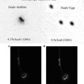
Modern confocal instruments are capable of detecting fluorescence emissions ranging from 400 to 700 nm. This covers a wide range of commonly available fluorescent probes. Spectral imaging systems either via multiple filters in a filter wheel or array of detectors with a spectral grating further aid the detection of probes with overlapping emission spectra and the imaging of more technically challenging specimens that may be compromised by autofluorescence that overlaps the emission wavelength of the probes of interest (Fig. 8). The AOTF is an invaluable aid to imaging multiple wavelength specimens since it affords fine control of both the intensity and the illumination wavelength at a high rate.