Fig. 5.1
Isotropic and anisotropic diffusion
Diffusion in biological tissues is affected by the microstructure of the respective tissue. In biological tissue, the water molecules still randomly diffuse in each 3D direction (isotropic) but are slowed down in their range due to collision with large-scaled biological molecules. Therefore, the diffusion coefficient for water in biological tissues, which is called apparent diffusion coefficient (ADC), is lower than in water. In an unorganized biological environment, ADC is independent from the direction of measurement, as a result of the spherical shape of diffusion. However, the radius of diffusion is reduced compared to unhindered diffusion when considering equal time points.
5.2.3 Anisotropic Diffusion
In highly structured biological tissues, such as white matter of the brain, the movement of water molecules is restricted by cell membranes, myelin sheaths, and microfilament (Jones et al. 2013). The diffusion probability of water molecules in structured tissue describes an ellipsoid based on the preferred diffusion direction parallel to the axon (Fig. 5.1b) (Basser et al. 1994a, b). In organized tissues such as the white matter, the ADC depends on the direction from which it is measured. The ADC is higher if the diffusion gradients are aligned to the preferred diffusion direction and lower if measured perpendicular to it.
5.3 Magnetic Resonance Diffusion-Weighted Imaging
5.3.1 Magnetic Resonance Imaging
Magnetic resonance imaging (MRI) relies on the nuclear spin which is innate to all elements with an odd-numbered composition of nuclear particles in their nucleus (Rabi et al. 1938). One example is the hydrogen nucleus consisting of a single proton. The proton can be understood as a charged moving particle while the conoidal movement as described by its spin axis is called precession (Loeffler 1981). Tissues of the human body contain between 22 % (bones) and 95 % (blood plasma) water and are therefore rich in protons. In a static magnetic field, the spins are precessing parallel and antiparallel to the magnetic field axis. Both orientations can be understood as different states of energy, where the upward spins are on a lower energetic level compared to the downward spins. In order to keep the energetic balance, there are more upward-oriented spins. The surplus of spins oriented upward causes a constant magnetization along the axis of the static magnetic field (z-axis which is also called longitudinal magnetization). MRI uses radiofrequency pulses to disrupt the constant magnetization and tilt the spin axis into the xy-plane (transversal magnetization) (Loeffler 1981). The moving sum of magnetic vectors in the xy-plane induces an alternating voltage in the reception coil (MRI signal). The process in which the transversal magnetization returns to the longitudinal magnetization is accompanied with energy loss and is called spin-lattice relaxation or T1-relaxation. In contrast the T2-relaxation is caused by energetic shifts between the spins while dephasing, while no energy is getting lost to the surrounding (Loeffler 1981).
5.3.2 Diffusion-Weighted Imaging
In diffusion-weighted imaging (DWI), the strength of the MRI signal depends on the mean displacement of water molecules. Here a strong signal indicates a low diffusion in the direction of the magnetic gradient field. Accordingly, the signal loss is higher when the mean displacement of the water molecules is higher along the gradient. The mean displacement of water molecules is described as the apparent diffusion coefficient (ADC). In the clinical setting, DWI is often used in the assessment of stroke (Warach et al. 1995; Brunser et al. 2013) because extracellular diffusion restriction due to the swelling of neurons is a highly sensitive marker of cerebral ischemia. This was first described by Moseley in 1990 (1990).
5.3.2.1 Stejskal-Tanner Sequence
To obtain diffusion-weighted images, the Stejskal-Tanner sequence is applied (Stejskal and Tanner 1965). A basic scheme of this sequence is given in Fig. 5.2. The process starts by applying a 90° radiofrequency pulse after time (t) to shift the magnetization vector into the xy-plane. The equal precessing spins create a magnetic momentum that is rotating in the xy-plane thereby inducing a voltage that can be referred to as the MRI signal. Due to intermolecular interactions and also due to field inhomogeneity, the first equally precessing spins start to diphase, resulting in a decay of the T2 signal. Now a 180° radiofrequency pulse is applied to turn the whole spin magnetization around. Previously slower precessing spins are now put ahead of faster precessing spins. After time (2 t = TE), all spins precess in phase again, and the recovered magnetic momentum induces a voltage, the spin echo. One could also state that by using the 180° pulse, the effect of field inhomogeneities is reversed. For diffusion weighting, two magnetic gradients are applied in addition to the static magnetic field and the radiofrequency pulse (Stejskal and Tanner 1965). Here the first linear gradient weakens or strengthens the local field strength resulting in a certain position-dependent precession frequency of corresponding spins. For spins in solid tissue, the effect of this gradient whether weakened or strengthened is reversed by the second gradient pulse (Stejskal and Tanner 1965). The signal loss is larger in tissues where the containing spins can move more rapidly between the applications of both gradient pulses.
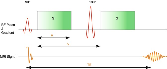
Fig. 5.2
Stejskal-Tanner Sequence
5.3.3 Diffusion Tensor Imaging
Diffusion tensor imaging (DTI) emerged from DWI in 1994 (Basser et al. 1994a, b). DTI is also based on the diffusion of water molecules as acquired with the Stejskal-Tanner sequence. The main advantage over DWI is that it makes it possible to quantify not only the diffusion in total but also the directionality of diffusion, which is called the diffusion tensor. In order to quantify the diffusion tensor, six different diffusion measurements and directions are necessary to sufficiently satisfy the tensor equation (Pierpaoli et al. 1996). Information content and reliability of the calculation of the diffusion tensor can be further improved by increasing the number of diffusion directions. Moreover, for complex post-processing analyses such as tractography, at least 30 diffusion directions are recommended in order to obtain reliable results (Spiotta et al. 2012). Increasing the number of diffusion directions enhances the precision of the reconstruction while the statistical rotational variance is reduced (Jones et al. 2013). The 3D information obtained from various diffusion gradients is used to calculate a multilinear transformation, the diffusion tensor. The diffusion tensor can be described using eigenvalues and eigenvectors and visualized as the diffusion ellipsoid (Fig. 5.3). The axes of the three-dimensional coordinate system are called eigenvectors, while the length of their measure is called eigenvalues. The three eigenvalues are symbolized by the Greek letter lambda (λ1, λ2, λ3). The eigenvalues are then used to calculate different parameters of the diffusion tensor.
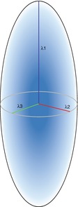
Fig. 5.3
Eigenvalues of the diffusion ellipsoid
5.3.4 Quantitative Parameters of the Diffusion Tensor
Commonly used quantitative parameters of the diffusion tensor are axial diffusivity (AD); radial diffusivity (RD); trace, mean diffusivity (MD); and fractional anisotropy (FA). These parameters are calculated for each voxel of the imaging data set and make it possible to characterize, noninvasively, tissue on a microscopic level.
5.3.4.1 Axial Diffusivity and Radial Diffusivity
The largest eigenvalue is named λ1 and is oriented parallel to the axonal structures. It is therefore equal to the diffusion tensor parameter axial diffusivity:

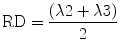
The eigenvalues λ2 and λ3 are the values along the two short axis of the coordinate system. They are therefore used to calculate the radial diffusivity which describes the diffusion perpendicular to the main diffusion direction. RD is calculated by dividing the sum of the short-axis eigenvalues by 2:
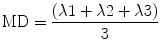
5.3.4.2 Trace and Mean Diffusivity
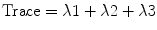
The sum of all three eigenvalues is called trace. Mean diffusivity is obtained when trace is divided by three:
5.3.4.3 Fractional Anisotropy
The calculation of fractional anisotropy weighs the preferred component of diffusivity to obtain information about the quantity of directionality. Therefore, the square root of the diffusion differ-ences 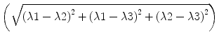 is used and then averaged by the square root of sums of squares
 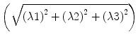 . The first term
  scales the FA to values between 0 and 1:

is used and then averaged by the square root of sums of squares . The first term scales the FA to values between 0 and 1:Based on these DTI parameters, assumptions can be made regarding the microstructure of the brain such as the orientation and diameter of axons and their surrounding structures such as the myelin sheaths. For example, decreased RD and therefore higher FA can be based on increased axonal density, reduced axonal diameter, and thicker myelin sheaths (Song et al. 2002). A lower FA can be caused by a number of factors, for example, a larger axon diameter (Takahashi et al. 2002), a lower axon density (Takahashi et al. 2002), and/or increased membrane permeability. Increased mean diffusivity represents an increase in extracellular diffusion of water molecules and can be the result of, for example, vasogenic edema (Filippi et al. 2001).
5.4 Post-Processing of DTI Data
5.4.1 Quality of DTI Data
The first and one of the most important steps in post-processing diffusion MRI data is to check the quality of the acquired data. The importance of the quality check arises from the susceptibility of diffusion MR images to artifacts, for example, motion artifact and/or susceptibility artifacts. While there are no strict guidelines for the post-processing of DTI data or standardized quality assurance, it is recommended that manual inspection be performed on the data, slice by slice, in order to ensure that reliable results are obtained for all acquired diffusion directions. All regions of interest must also be free from any artifact to avoid possible confounds in the calculation of diffusion parameters.
5.4.2 Diffusion Tensor Masks
Most post-processing techniques require a mask for the individual data set that contains only the brain and the surrounding cerebrospinal fluid (CSF) space. These masks can be obtained automatically using a software such as the brain extraction tool (BET), which is part of the FSL software (FMRIB Software Library, The Oxford Centre of Functional MRI of the Brain – FMRIB). To guarantee a high quality of data and to take the individual’s anatomy into account, the masks created automatically are then manually edited. The latter can be a labor-intensive process.
5.4.3 Visualization of DTI Parameters
The easiest way to visualize the DTI parameters is by displaying the value as the level of gray in each respective voxel (Fig. 5.4a). By adding the information of the main diffusion direction using a color scheme, color-coded maps can be obtained (Fig. 5.4b). Blue-colored voxels represent the main diffusion direction parallel to the z-axis, that is, inferior to superior in human individuals. In contrast, the green-colored voxels represent the main diffusion direction parallel to the y-axis, that is, anterior to posterior. Red-colored voxels represent a main diffusion direction parallel to the x


Related posts:

Stay updated, free articles. Join our Telegram channel
Full access? Get Clinical Tree
