Fig. 6.1
Representative proton spectrum acquired from the posterior cingulate gyrus. Data were acquired using a 3 T clinical MRI scanner and point-resolved spectroscopy localization with an echo time of 30 ms and repetition time of 2 s. Voxel location is shown in the inset to the right in the axial, coronal, and sagittal planes. Major metabolites of N-acetylaspartate (NAA), glutamate and glutamine (Glx), creatine (Cr), choline (Cho), and myoinositol (mI) are labeled
Each chemical resonates at established frequencies that upon Fourier transform results in peaks at specific locations, or chemical shifts, along the x-axis. The chemical shift of each chemical is governed by the structure of the chemical, in particular, the grouping of the hydrogen atoms as single or multiple peaks (singlets and multiplets), and proximity to other hydrogen-containing groups (J-coupling). These chemical shifts are often expressed as “parts per million,” which can be confusing as it does not relate to the concentration of the chemical, but historically has been used to express the frequency. The use of this nomenclature is so that it is not dependent upon the field strength of the magnet used such that the resonance frequencies are the same between a 1.5 T MRI scanner and a 3.0 T scanner. The concentration of the metabolite is expressed along the y-axis as the height of the peak such that higher concentrations result in higher peaks and vice versa. Quantitation of these peak heights can provide an objective measure of brain biochemistry that is similar to a blood test or lab analysis: different concentrations are measured and reported, which can then be used for diagnosis or disease characterization. More importantly, however, the role of each of the chemicals is tied to metabolic and physiological processes within the brain that directly relate to cognitive or neuronal processes. The remainder of this chapter will be devoted to the major metabolites that are detected by MRS, as well as the different methods by which the data can be collected.
6.2 N-Acetylaspartate (NAA): Neuronal Marker
As indicated in the spectra in Fig. 6.1, one of the chemicals that can be measured by MRS is NAA. The primary resonance of NAA is at 2.02 ppm. It is an amino acid derivative synthesized in neurons and transported down axons. It is therefore a putative “marker” of viable neurons, axons, and dendrites. Studies where NAA was labeled with fluorescent tags demonstrated that NAA was distributed throughout the neuron and axon (Moffett et al. 1993). Studies have also correlated the concentration of NAA in the brain with the number of neurons measured (Urenjak et al. 1992). The ability to quantifiably measure neuron populations allows MRS to provide a diagnostic tool that no other radiological technique can match: an ability to literally “count” the number of active brain cells using a completely noninvasive and quantitative technique by simply measuring the peak height of the NAA chemical in the MRS spectra. This can be utilized in a number of practical means. For example, every metabolite has a “normal” concentration that generates a pattern of peaks that is the same from person to person unless there is an underlying pathology. Diagnosis with MRS can therefore be made either by comparing the numeric values of metabolite concentrations or by recognizing abnormal patterns of peaks in the spectra. With either method, it is the increase or decrease in the concentrations of the metabolites that is diagnostic for pathology as has been shown across a broad variety of diseases (Lin et al. 2005; Harris et al. 2006; Moffett et al. 2007). However, it should also be noted that NAA is a cerebral metabolite that participates in a number of metabolic processes, and therefore, the interpretation of NAA as solely a neuronal marker is somewhat of an oversimplification (Barker 2001). It is important to understand the context of NAA metabolism, as detailed below.
6.2.1 NAA Metabolism
NAA is formed by the transamination of glutamate (Glu)with oxaloacetate which leads to aspartate (Asp) (Cooper et al. 1970), and in the presence of acetyl coenzyme A and NAA synthase, (l-aspartate N-acetyltransferase), aspartate (Asp) is converted to NAA. This process occurs primarily, but not exclusively, in neurons, where it exhibits a very high intracellular–extracellular gradient. NAA is hydrolyzed back into aspartate and acetate by aspartoacylase (N-acetyl-l-aspartate amidohydrolase) in mature oligodendrocytes only. In some neurons, a portion of NAA is turned into N-acetylaspartylglutamate (NAAG) in the presence of glutamate (Glu) by an NAAG synthase (N-acetylaspartate-l-glutamate ligase) (Baslow 2000). NAA and NAAG are major neuronal osmolytes, and the large amount of NAA and NAAG present in the brain can serve as cellular reservoirs for Asp and Glu. Since both are polar and ionizable hydrophilic molecules that undergo a regulated efflux into extracellular fluid, they can also play a role in water movement out of neurons (Baslow 2000). In addition, the fact that the NAA-metabolizing enzyme aspartoacylase is an integral component of the myelin sheath suggests that intraneuronal NAA may supply the acetyl groups for myelin lipid synthesis (Chakraborty et al. 2001). Finally, the cell type-specific metabolic enzymes in the NAA and NAAG cycle indicate a three-cell compartmentalization involving neurons, astrocytes, and oligodendrocytes. Those neurons that may synthesize NAAG from NAA and Glu target the release of NAAG to astrocytes, where it is cleaved into NAA and Glu. The Glu is taken up by astrocytes, where it may be returned to neurons via the glutamate–glutamine cycle. The residual NAA extracellular products are removed and hydrolyzed by oligodendrocytes (Baslow 2000). This unique tricellular metabolic cycle, as shown in Fig. 6.2, involving NAA and NAAG, provides a potential glial cell-specific signaling pathway, which can also be reflected in changes in different diseases (Baslow 2010).
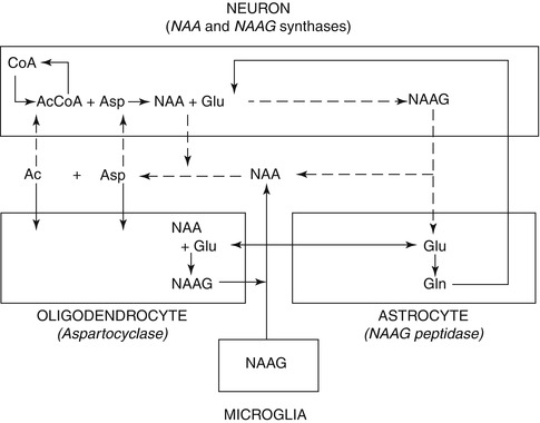
Fig. 6.2
Tricellular NAA–NAAG cycle operating between neurons, astrocytes, and oligodendrocytes (Modified from Baslow 2010). CoA coenzyme A, Acetyl-CoA acetyl coenzyme A, Asp aspartate, Glu glutamate, Gln glutamine, NAA N-Acetylaspartate, NAAG N-Acetylaspartylglutamate
6.2.2 Measuring NAA Using Single Voxel Spectroscopy
As a “virtual biopsy,” localization is required when examining specific regions of the brain involved in disease. Localization is defined by a region of interest, or voxel, from which the spectrum is acquired and, hence, described as single voxel spectroscopy (SVS). This region is a cube within the brain that can be visualized and placed in the sagittal, coronal, and axial planes as shown in Fig. 6.1. The localization is achieved by utilizing a pulse sequence that acquires the MRS signal. Though several sequences, and permutations of sequences, exist which are capable of yielding an in vivo MRS spectra, many of them are research techniques and not widely available (although discussed later in this chapter). The two most commonly used sequences are PRESS and STEAM as described below:
6.2.2.1 Point-Resolved Spectroscopy (PRESS)
The point-resolved spectroscopy (PRESS) sequence is a standard part of the software package that accompanies the two most popular MRI manufacturers, Siemens (Erlangen, Germany) and General Electric (Waukesha, Wisconsin). On Siemens scanners, it is known as “svs_se.” On General Electric machines, the sequence is called “Probe-P.” The PRESS sequence was originally developed in 1987 by Paul Bottomley at General Electric (Bottomley 1987) and utilizes three orthogonal magnetic field gradients along the x-, y-, and z-axes using slice-selective 90° pulse followed by two slice-selective 180° pulses to select a specific three-dimensional voxel, within which a proton MRS spectrum can be obtained.
6.2.2.2 Stimulated Echo Acquisition Mode (STEAM)
STEAM also uses a series of three consecutive slice-selective 90° pulses for localization. However, the sequence only yields half as much detectable magnetization; therefore, the signal-to-noise ratio is halved. Nonetheless, adequate water suppression—which is necessary for all MRS techniques, as the metabolites to be detected exist at much lower concentrations than water—is more easily accomplished via STEAM (Haase et al. 1986). Shorter echo times are also attainable with STEAM, which may provide an advantage when detecting short T2 metabolites such as γ-aminobutyric acid (GABA).
6.2.2.3 Post-processing Single Voxel Data
SVS data can be post-processed and analyzed in several different ways. All major MR platforms have their own methods of reconstructing the data where the details are somewhat different, but the end result is generally an automated or semiautomated fitting of the metabolite peaks and a quantitative measure of major metabolites (NAA, creatine, choline, myoinositol), usually as a ratio to creatine to provide a normalization factor to account for differences in the peak area or amplitude between subjects which will differ depending on parameters such as the voxel size, number of averages, transmit gain, etc. The MRS data can also be exported for further analysis using MRS post-processing packages such as LCModel (Provencher 1993), jMRUI/AMARES (Vanhamme et al. 1997), etc. The advantage of this more sophisticated post-processing is that it allows for “absolute quantitation” of the metabolites by incorporating prior knowledge or additional measures (Kreis et al. 1993) that provide a concentration in millimolar per kilogram wet weight that would be equivalent to in vitro measurements of metabolite concentrations. While the accuracy of the quantitation, in terms of “absolute” quantitation, is somewhat controversial, the advantage of this method is that the metabolites can be quantified without being a ratio to creatine. This is especially important in diseases that can cause a change in creatine, in which case it is unclear whether it is the major metabolite that has altered or creatine or both.
6.2.3 Measuring NAA Using Chemical Shift Imaging (CSI)
One of the drawbacks of SVS is the natural limits of a single area of acquisition. Obtaining spectra in many different areas of the lesion would be time consuming. Multivoxel spectroscopy, also called chemical shift imaging (CSI) or spectroscopic imaging, overcomes this issue by adding an additional phase-encoding step that allows for spatial encoding of a larger volume such that it is divided into smaller voxels that can be summed or selected chemical shifts can be color-coded into chemical shift maps. In experimental duration, some two to three times longer than that in which a single voxel method acquires the spectrum of a single ROI, the CSI technique (Maudsley et al. 1983) can collect an array of spectra from a single plane.
6.2.3.1 CSI Pulse Sequence
STEAM and PRESS are still utilized for localization; however, phase-encoding gradients are employed to encode the spatial dimensions, and the MR signal is collected in the absence of any gradient in order to maintain the spectroscopic information. Each acquired ROI contains an MR spectrum that allows for the assessment of the metabolic profile of a specific location or allows for visualization of the spatial distribution of specific metabolites of interest. CSI also allows for the acquisition of smaller volumes than in single voxel techniques (as small as 0.4 cm3 at higher magnetic field strength). This has the advantage over single voxel MRS techniques, as multiple brain regions can be assessed using the CSI technique which can also be completed offline via post-processing routines that allow for positioning of different areas of interest, assuming that they are contained with the larger region of interest selected for CSI acquisitions. Furthermore, there are additional variants of CSI that utilize different phase-encoding methods to either reduce scan time or allow for additional spatial resolution and information such as spiral phase encoding, echo planar sequences, multislice sequences, and parallel imaging methods (Posse et al. 2013).
6.2.3.2 Reconstruction of CSI Data
The main advantage of CSI is that the spatial information is retained such that during post-processing one can characterize the spectra in a number of different methods. The field of view can be partitioned into individual voxels determined by the resolution of the phase encoding. For example, if 16 frequency encodes and 16 phase encodes are used in a 16-cm2 field of view and 1-cm slice thickness, each voxel will have a resolution of 1 × 1 × 1 cm3, and a spectrum can be reconstructed in each voxel as shown in Fig. 6.3a. Analyzing each voxel would be time consuming, and therefore, there are two different ways to display the data. First, one can create a “metabolite map” which selects a certain region of the spectrum, for example, 2.0–2.05 ppm for NAA, which creates a map based on the signal intensity of the spectrum from that spectral region, which is then displayed on top of the MRI image as shown in Fig. 6.3b. The spatial resolution of the metabolite maps are often interpolated which may result in over-interpretation of the true voxel resolution. There are also issues with signal correction where some areas may appear to have increased SNR but overall signal may be increased in that region, leading to possible misinterpretation of the data. It is therefore somewhat dangerous to rely solely on metabolite maps without evaluating the individual spectra. One can sum all of the spectra from a certain region of the spectrum, much like a single voxel acquisition as shown in Fig. 6.3c. This procedure is repeated at multiple regions in the CSI volume. The major advantage of CSI is that in post-processing, the ROI can be readily shifted to any location with the excitation volume.
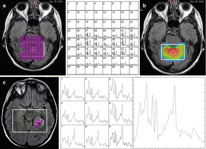
Fig. 6.3
Representative chemical shift imaging. (a) Left: MRI image with grid of voxels indicated in purple. Right: reconstruction of CSI data as individual spectra. (b) Metabolite map of NAA. (c) Simplified display of CSI data as a small grid of spectra as indicated on the image (left) and individual spectra (middle) and summed spectra (right)
However, CSI suffers from the disadvantage that the shape of individual ROIs is less well defined than in single voxel techniques. This can result in the adjacent ROIs being contaminated by large-amplitude signals from surrounding ROIs. Furthermore, CSI is not as reproducible as SVS (Rosen and Lenkinski 2007) and therefore is less sensitive to the more subtle changes. Finally, on most clinical scanners, the majority of CSI acquisitions are set up for long echo MRS which also eliminates important diagnostic metabolites such as glutamate Glu or myoinositol (mI), although for NAA, the focus of this section, it is sufficient.
6.2.4 Whole-Brain NAA
As described above, single voxel and CSI methods suffer from issues such as lipid contamination, voxel registration, as well as assumptions of T1 and T2 relaxation times. One method of addressing the aforementioned issues is to take advantage of the fact that NAA is the most prominent peak within the MRS spectrum (thus having a high signal-to-noise ratio) that acquires signal from the entire head and is thus named whole-brain NAA (WBNAA) spectroscopy (Rigotti et al. 2007). Unlike the single voxel and CSI methods, WBNAA does not utilize localization and instead acquires data immediately after excitation (TE = 0 ms) with a very long repetition time (TR = 10 s) and a short inversion time (TI = 940 ms). The inversion pulse is alternated between each acquisition where the TI is designed to null the NAA signal. The even and odd acquisitions are then subtracted from one another which nulls those metabolites, including lipid, that have a short T1 relaxation time. As NAA has a long T1 relaxation time (1.4 s), it remains visible. As a result of the long TR, there are no T1- or T2-weighting effects. The WBNAA signal is then normalized to the total brain volume as can be obtained from brain segmentation. This method operates under the assumption that all NAA arises from within the brain, and given the lack of localization, results of such studies would imply global effects of the disease.
6.2.5 NAA in Psychiatric Diseases
6.2.5.1 Schizophrenia
A recent meta-review of spectroscopy papers in schizophrenia revealed 103 papers alone that focused on MRS which included a total of 2,067 subjects and 2,115 controls of which the great majority of the studies focused on treated chronically ill patients (Kraguljac et al. 2012). All papers utilized either the SVS or the CSI methods, thereby allowing for regionalized differences to be measured. Decreased levels of NAA were found all across the brain including structures such as the hippocampus, thalamus, and frontal and temporal lobes. While the temporal lobes showed the greatest decreases in NAA with a standardized mean difference of −0.72, the variability of measurements in the temporal lobe were also greater than any other area of the brain. The reason for this variability is due to the susceptibility artifacts that occur due to the air and bone tissue interfaces within this brain region that result in distortions and signal loss (Olman et al. 2009). The basal ganglia and frontal lobe showed the most consistent decreases in NAA. While WBNAA measures have not been applied to schizophrenia, these global changes in NAA throughout the schizophrenic brain would indicate that this method would be sensitive to these changes.
6.2.5.2 Dementia
Given the relationship between NAA and neuronal viability, NAA is a key biomarker for dementia. Dozens of papers have shown decreases in NAA in both cortical and white matter regions of the brain including the posterior cingulate gyrus, the temporal lobe, and the occipital lobe (Graff-Radford and Kantarci 2013). In combination with myoinositol (mI), a putative glial marker, NAA provides up to 90 % sensitivity and 95 % specificity for distinguishing Alzheimer’s disease (AD) from healthy subjects (Kantarci 2007). In a recent study, the ratio of NAA/mI predicted progression to mild cognitive impairment (MCI) or dementia in 214 subjects (Kantarci et al. 2013), which supports previous findings of reduced NAA in MCI patients. Furthermore, MRS is valuable in differentiating between different types of dementia such as the Lewy body, frontal lobe, and vascular dementia (Shonk et al. 1995; Kantarci et al. 2004). While the temporal lobe is often thought to be the ideal location for detecting Alzheimer’s disease, it is the posterior cingulate gyrus that has been shown to be the most sensitive to AD. While there may be a neuropathological role for the posterior cingulate cortex in AD, as has been shown in PET studies (Minoshima et al. 1997), this region of the brain is also one of the most homogeneous parts of the brain that results in spectra of superior technical quality, which would also contribute to the diagnostic sensitivity of MRS to AD and other dementias.
6.2.5.3 Depression/Bipolar Disorder
Changes in NAA in bipolar disorder and major depression have also been studied extensively (Capizzano et al. 2007). Several studies have shown reductions in NAA/Cr in the temporal lobes as a result of bipolar disorder. Some studies have also shown reductions in NAA/Cr in the frontal lobe in patients suffering from major depression; however, there are also studies that were not able to replicate these results. This may be due to the fact that a majority of the studies used a ratio to Cr despite the fact that some studies have shown that Cr is altered as a result of major depression (Gruber et al. 2003).
6.3 Glutamate: Excitatory Neurotransmitter
Glutamate (Glu) is an amino acid with several important roles in the brain. First, it is the most abundant excitatory neurotransmitter in the human brain, where it plays a major role in neurotransmission and where it is released from presynaptic cells and then binds to postsynaptic receptors, thus inducing activation as shown in Fig. 6.4. As a result, many neurological and psychiatric diseases have an impact upon Glu. In particular, dysfunction reflected in excessive Glu release or reduced uptake can lead to an accumulation of Glu, which results in excitotoxicity. This second mechanism is key to not only understanding the underlying pathophysiology of different brain disorders but also providing a potential pathway for disease treatment. The existence of numerous Glu agonists and antagonists now allows for pharmaceutical interventions that can be used to modulate glutamate Glu levels and thus provide potential treatments. Finally, Glu is a key compound in brain metabolism via the citric acid cycle and therefore also tightly coupled to brain energetics.
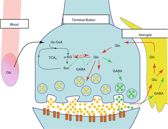
Fig. 6.4
Glutamate cycle in the neuron and glia. Glucose (Glc) from the capillaries is the primary source of fuel for the neurons which are then metabolized via the tricarboxylic acid cycle (TCA) to acetyl coenzyme A (acetyl-CoA), then to alpha-ketoglutarate (α-KG), and finally to succinate (Suc). α-KG is transaminated to glutamate (Glu), which can be further metabolized to gamma-aminobutyric acid (GABA). However, it is primarily released by the neuron and then taken up into the astroglia and metabolized to glutamine (Gln)
6.3.1 Glutamate and Glutamine Metabolism
Metabolically, glutamate (Glu) is stored as glutamine (Gln) in the glia, and the balanced cycling between these two neurochemicals is essential for normal functioning of brain cells. Glu and Gln are compartmentalized in neurons and glia, respectively, and this chemical interconversion reflects an important aspect of metabolic interaction between these two types of cells. In vivo studies have revealed that the neuronal/glial Glu/Gln cycle is highly dynamic in the human brain and is the major pathway of both neuronal Glu repletion and astroglial Gln synthesis (Gruetter et al. 1994; Mason et al. 1995). After its release into the synaptic cleft, Glu is taken up by adjoining cells through excitatory amino acid transporters. Astrocytes are responsible for the uptake of most extracellular Glu via Glu transporters and additionally have a vital role in preserving the low extracellular concentration of Glu needed for proper receptor-mediated functions, as well as to prevent excitotoxicity (Schousboe 2003; Schousboe and Waagepetersen 2005). Once taken up into the astrocyte, Glu is rapidly converted to Gln by the enzyme Gln synthetase. Small quantities of Gln are also produced de novo or from GABA (Hertz and Zielke 2004; Bak et al. 2006). Gln is released from astrocytes, accrued by neurons, and converted to Glu by the neuron-specific enzyme phosphate-activated glutaminase (Bak et al. 2006). Gln is the main precursor for neuronal Glu and GABA (Hertz and Zielke 2004), but Glu can also be synthesized de novo from tricarboxcylic acid cycle intermediates (De Graaf et al. 2011). The rate of Glu release into the synapse and subsequent processes are dynamically modulated by neuronal and metabolic activity via stimulation of extrasynaptic Glu receptors, and it has been estimated that the cycling between Gln and Glu accounts for more than 80 % of cerebral glucose consumption (Sibson et al. 1998). The tight coupling between the Glu/Gln cycle and brain energetics is largely tied to the nearly 1:1 stoichiometry between glucose oxidation and the rate of astrocytic Glu uptake. This relationship was first determined by Magistretti et al. in cultured astroglial cells where the addition of Glu resulted in increased glucose consumption (Pellerin and Magistretti 1994). These results provided the hypothesis that glycolysis in the astrocytes results in a production of two molecules of ATP, which are then consumed by the formation of Glu from Gln, which suggests a tight coupling between the two mechanisms.
6.3.2 Glutamate and Glutamine Structure and Spectroscopy
The molecular structures of Glu and Gln are very similar and, as a result, give rise to similar magnetic resonance spectra (Govindaraju et al. 2000). The four protons from the two methylene groups of glutamate Glu and Gln are located at 2.04–2.35 ppm and 2.12–2.46 ppm, respectively. Similarly, the methine group resonates at 3.74 ppm and 3.75 ppm for glutamate Glu and Gln, respectively. Thus, even though Glu has a relatively high concentration in the brain, its major resonances are usually contaminated by contributions from Gln, GABA, glutathione (GSH), and NAA. To avoid confusion in spectral assignment of Glu and Gln, the term “Glx” has traditionally been used to reflect the combined Glu and Gln concentrations. However, this approach does not allow for the evaluation of conditions where the concentrations of Gln and Glu are in opposing directions, nor does this approach allow for the evaluation of Gln and Glu separately. As our understanding of the importance of Glu/Gln system in the human brain has increased, much endeavor has been invested in being able to quantify Glu or Gln separately. The sections below detail methods for measuring Glu utilizing various pulse sequences to achieve the separation of Glu from co-resonating metabolites.
6.3.3 Single Voxel MRS and LCModel
LCModel (Provencher 1993) is a software package often used for post-processing of MRS data. It utilizes prior knowledge in the form of a basis set that is made up of a linear combination of in vitro, or simulated, spectra from individual metabolite solutions. The advantage of this method is that it is almost completely automated and utilizes algorithms for baseline correction and peak fitting without imposing restrictive parameterization and without subjective input. It is often used in the literature to calculate concentrations of individual metabolites including Glu and Gln. LCModel provides a quantitative measure of the accuracy of the measure by using the estimated standard deviations or Cramer–Rao lower bound (CRLB) that provides a measure of how reliable the measurement is. A standard deviation of <20 % has been used throughout the literature as the criteria for adequate reliability. While Glu standard deviation measures tend to fall below 20 %, Gln standard deviation measures do not. Given the overlap between the two molecules, it is unclear whether LCModel can accurately discern Glu from Gln.
In our lab we conducted a series of experiments where different solutions, or phantoms, were created that had different concentrations of Glu and Gln. In three of the phantoms, Glu was increased from 6 to 18 mM concentrations and Gln was maintained at 6 mM, which is equivalent to the physiological concentrations in the brain (3–5.8 mM (Govindaraju et al. 2000)). In the other three phantoms, Glu was maintained at 12 mM (equivalent to in vivo concentrations of 6–12.5 mM (Govindaraju et al. 2000)), but Gln was increased from 3 to 12 mM. Spectra were then acquired from these solutions using a clinical MRI scanner (Siemens 3 T TIM Trio) using conventional PRESS MRS (echo time of 30 ms, repetition time of 2 s). LCModel was then used to calculate the concentrations of each phantom as shown in Fig. 6.5. Our results showed that the variable concentration of Gln has a direct effect on the reported Glu concentrations and therefore demonstrates that this method is not sufficient for discerning Glu from Gln.
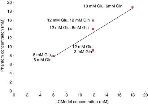
Fig. 6.5
Titration curve of solutions of glutamate and glutamine. Different concentrations of glutamate and glutamine were created as indicated by the data labels. The results show that the different concentrations of glutamine had a strong effect on the 12-mM Glu phantom solutions such that LCModel over- and underestimated the Glu concentration when Gln concentrations were high and low, respectively
6.3.4 Optimal Echo Time
In order to better separate Glu and Gln, the echo time can be altered to minimize the contribution of the Gln signal to the Glx complex. Schubert et al. (Schubert et al. 2004) were able to selectively detect C4 proton resonances of Glu using a PRESS sequence at 3 T with a TE of 80 ms and analyzing the data using both the time and the frequency domains with prior knowledge obtained from phantom spectra. Using this approach, in vivo spectral features were similar to in vitro Glu spectral features collected from a phantom, and Glu signal was well resolved and separated from major interferences, such as Gln and NAA. Similarly, Jang et al. acquired PRESS spectra at 1.5 T in vitro and in vivo at four TE values: 30, 35, 40, and 144 ms (Jang et al. 2005), with the resulting spectra analyzed with LCModel (Provencher 2001). In vitro and in vivo spectra yielded the lowest Cramer–Rao lower bounds (CRLB) for Glu quantitation when TE was set to 40 ms. TE optimization for the purpose of Glu and Gln detection has also been demonstrated using stimulated echo acquisition mode (STEAM) spectroscopy by Yang et al. (2008), who optimized TE and mixing time (TM) to resolve the C4 proton resonances of Glu and Gln. Optimal TE methods are appealing acquisition strategies due to their ease of implementation for both acquisition and processing and the ease with which appropriate parameter timings can be selected at the scanner interface. Additionally, the resulting spectra can be analyzed using scanner software or commercially available software (e.g., LCModel, jMRUI) after simulating an appropriate basis set.
6.3.5 Ultrashort Echo Time
Due to the fact that Glu is a strongly coupled system, short echo time acquisitions are usually preferred over long echo time acquisitions for the purpose of reducing peak phase modulation. The ultrashort TE approach in such coupled systems gives rise to spectra where the majority of peaks are inphase and thus reduces signal cancellations due to J-modulations at longer echo times which in turn lead to more robust signal quantification. Wijtenburg and Knight-Scott (2011) quantified Glu/tCr at 3 T by combining short TE STEAM (6.5 ms) with phase rotation (Hennig 1992; Ramadan 2007) to detect Glu in human brain. This approach has been compared to 40 ms TE PRESS, 72 ms TE STEAM, and TE averaging and demonstrated that the short TE phase-rotation-STEAM approach yielded the greatest precision for Glu/tCr ratio quantification followed by TE averaging, PRESS 40 ms, and STEAM 72 ms (Wijtenburg and Knight-Scott 2011).
The implementation of very short echo time techniques requires substantial modification of standard vendor-supplied localization sequences. These spectra are usually complicated by a broad baseline extending over the whole spectral width, and care should be taken during analysis to eliminate the contribution of the baseline to the desired metabolite signal—which is usually done by utilizing T1 differences (Starcuk et al. 2001). The use of third-party spectral analysis software and, in some cases, the collection or simulation of metabolite basis set are essential to yield results of high accuracy (Wijtenburg and Knight-Scott 2011).
6.3.6 TE-Averaged PRESS
In this method, a number of 1D PRESS spectra are acquired at variable TE values and co-added (averaged) in real time to produce a single 1D, TE-averaged spectrum. Alternatively, the same TE-averaged spectrum can be obtained if these time-domain FIDs are ordered in a 2D matrix and a two-dimensional Fourier transform (2DFT) applied. The resultant 1D spectrum corresponding to the middle of the F1 axis (F1 = 0 Hz) is equivalent to the TE-averaged spectrum obtained above (Dreher and Leibfritz 1995; Bolan et al. 2002). This 1D spectrum offers relatively uncontaminated spectral peaks for C4 protons at 2.35 ppm for Glu and for C2 at 3.75 ppm for Glx (Hurd et al. 2004). Representative spectra are shown in Fig. 6.6a.
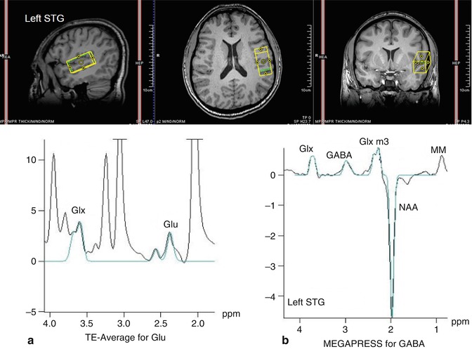
Fig. 6.6
In vivo spectra of schizophrenia. Representative spectrum of (a) glutamate-edited MRS (left panel) and (b) GABA-edited MRS (right panel) in the left superior temporal gyrus (STG) of a schizophrenia subject
While TE averaging is a simple and reliable method for measuring Glu and Gln, it sacrifices spectral information arising from the J-evolution of other metabolites. The method also suffers from differential T2 weighting per individual TE value, which can be corrected for if a basis set is similarly simulated or experimentally acquired. TE-averaging sequences are not usually available from major MRI vendors but can be easily modified from standard PRESS sequence source code.
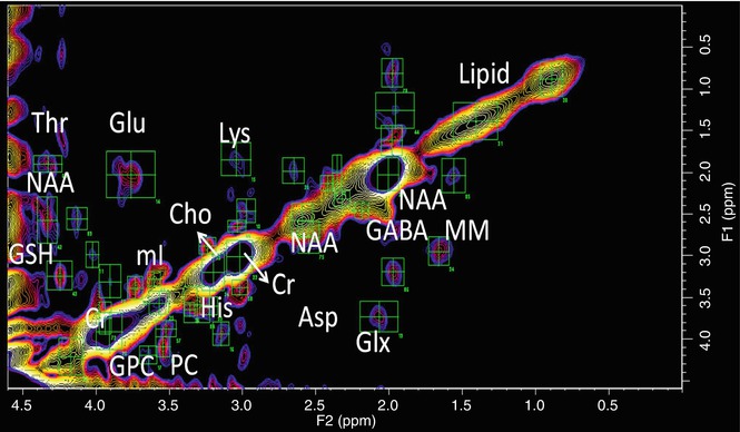
Fig. 6.7
2D correlated spectroscopy (COSY) of schizophrenia. Representative 2D COSY of left STG of SPD. Green ROIs show identification of multiple cross peaks such as threonine (Thr), N-acetylaspartate (NAA), glutathione (GSH), glutamate (Glu), myoinositol (mI), glycerophosphorylcholine (GPC), phosphorylcholine (PC), total choline (Cho), lysine (Lys), histidine (His), creatine (Cr), aspartate (Asp), gamma-amino butyric acid (GABA), glutamate–glutamine (Glx), macromolecules (MM), and lipids
6.3.7 Glutamate Chemical Exchange Saturation Transfer (GLuCEST)
A large sensitivity enhancement for the detection of Glu can be achieved by careful design of MR exchange experiments. A recent example of this technique was recently implemented by Cai et al. where the chemical exchange saturation transfer (CEST) between bulk water and Glu was utilized for the detection of Glu (Cai et al. 2012). In such CEST experiments, advantage is taken from the protons on the Glu amine group, which are labile and in constant exchange with the protons of bulk water. When the Glu NH2 protons are saturated by RF irradiation at 7.7 ppm (i.e., 3 ppm higher than water), the resultant saturation effect is transferred to water due to the ongoing chemical exchange between the protons of NH2 and H2O. This in turn leads to a reduction in the amplitude of water resonance due to the saturation of its protons and the saturation RF field applied to the Glu amine group. An excellent review of chemical exchange methodology can be found here (Zhou and van Zijl 2006).
6.3.8 Two-Dimensional MRS
An alternative to separating Glu from Gln is to use a second chemical shift dimension: 2D Fourier NMR spectroscopy utilizes a simple two-pulse sequence, 90x-t1-90x-Acq(t2), creating a dataset that is a series of one-dimensional (1D) spectra with traditional time readout (t2), but each with increments in delay (t1), inserted before the terminal readout 90° RF pulse (Jeener et al. 1979). Two-dimensional Fourier transformation (FT) of t1 and t2 produces a 2D spectrum where the x- and y-axes are the frequencies F2 and F1, respectively, known as correlated spectroscopy (COSY). In a 2D COSY spectrum, scalar coupling between protons in molecules results in cross peaks that allow for unambiguous identification of different metabolites (Thomas et al. 2001; Cocuzzo et al. 2011; Ramadan et al. 2011). This technology has been translated to clinical MR scanners and has been applied in vivo (Schulte et al. 2006), demonstrating detection of GABA, Glu, Gln, glutathione, as well as other metabolites (Fig. 6.7).
6.3.9 13C Spectroscopy
While the aforementioned methods have been utilized throughout the literature to study Glu, these measures provide static measures of Glu, measuring the total concentration of Glu in the brain without a sense of the dynamic changes that result from neurotransmission and brain energetics. Carbon 13 (13C) MRS is presently the only method that provides noninvasive measurements of neuroenergetics and neurotransmitter cycling in the human brain. 13C MRS, combined with the administration of 13C-labeled substrates, allows the detection of 13C incorporation from 13C-labeled precursors into various carbon positions of metabolites, including the Glu cycles between neuronal and glial compartments (De Graaf et al. 2011). For example, if glucose, the primary fuel for the brain, is labeled with a nonradioactive isotope of 13C on the first carbon, that label is retained as it is metabolized through the TCA cycle. At the point of alpha-ketoglutarate, the label is transaminated to Glu and Gln via the Glu/Gln cycle as shown in Fig. 6.8. As the label is incorporated separately into the fourth carbon group of Glu and Gln, real-time acquisition of the brain will result in the observation of the Glu C4and Gln C4 resonances at 34.4 ppm and 31.8 ppm, respectively. In the second turn of the TCA cycle, Glu C2 and C3 are labeled. Thus, 13C MRS allows continuous, noninvasive monitoring of metabolic fluxes under different physiological or pathophysiological conditions.
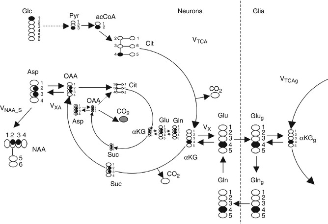
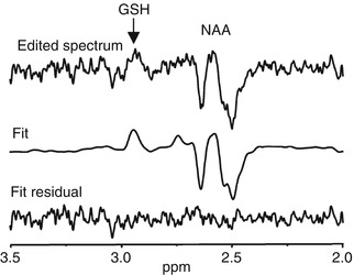
Fig. 6.8
Fate of 1-13C atom of glucose through neuronal TCA and part of the neuronal–glial glutamate–glutamine cycle involved in glutamate neurotransmission. Two turns of the TCA cycle are represented. Carbon atoms enriched are shown in black. Carbons with 50 % chance of enrichment are shaded. For clarity the 3rd turn of neuronal TCA is represented only by bicarbonate (13CO3) release. In the paper, 13CO2 is referred to as a bicarbonate (H13CO3). Other abbreviations: Glc glucose, Pyr pyruvate, acetyl-CoA acetyl coenzyme A, Cit citrate, V TCA tricarboxylic acid cycle rate, αKG 2-oxoglutarate, Vx ,αKG Glu transaminase rate, V XA )transaminase or malate–aspartate shuttle rate, Glu glutamate, Glug glial glutamate, Gln glutamine, Glng glial glutamine, αKGg glial 2-oxoglutarate, Suc succinyl CoA, OAA oxaloacetate, Asp aspartate, NAA N-acetylaspartate, V NAA_S NAA synthesis rate
Fig. 6.9
MEGA-PRESS GSH spectrum. Representative spectrum of glutathione measured by MEGA-PRESS. The difference spectrum is shown at the top, with an arrow pointing to the GSH resonance. The middle spectrum shows the fit of the data and the bottom spectrum shows the residual. Note the NAA is co-edited with this implementation of the MEGA-PRESS sequences (Terpstra et al. 2005)
The 13C MRS acquisition consists of several different steps providing multiple means by which Glu can be measured. These include choice of substrate (glucose, acetate, label position), method of delivery (oral, IV, glucose clamped), data acquisition (direct detection, indirect detection), and method of analysis (dynamic difference spectroscopy, isotopomer analysis) (Ross et al. 2003). It is important to note that the natural abundance of 13C is approximately 1.1 % which implies that there is very little background signal of indigenous 13C Glu, therefore providing excellent contrast to noise ratio of signals that arise from the incorporation of the 13C label via the TCA cycle and subsequent transamination from alpha-ketoglutarate to the Glu/Gln cycle.
6.3.10 Glutamate in Psychiatric Diseases
6.3.10.1 Schizophrenia
It is thought that schizophrenia is related to a dysfunction in N-methyl-d-aspartate (NMDA) receptors, the major subtype of Glu receptors. Evidence from studies of NMDA receptor agonists such as phencyclidine and ketamine has shown decreased Glu levels as well as the psychotic symptoms observed in schizophrenia (Javitt and Zukin 1991). A recent meta-review (Marsman et al. 2013) examined 28 publications for a total of 647 patients with schizophrenia compared with 608 healthy controls appears to support this hypothesis by showing evidence of reduced Glu. While several brain regions were explored including the medial frontal region, hippocampus, and thalamus, only significant differences were found in the medial frontal region with reduced Glu. Group-by-age associations showed that Glu decreased at a faster rate with age in patients with schizophrenia compared to controls. While there have been few longitudinal studies of Glu using MRS, the literature appears to reflect that first-episode schizophrenics show increased glutamate whereas in the chronic stage of disease, Glu is decreased (Port and Agarwal 2011). This provides the basis for the second hypothesis of excitotoxicity of Glu in schizophrenia. Proponents argue that initially Glu levels are increased leading to excitotoxicity, which in turn leads to neuronal death as reflected by decreases in NAA. In the chronic stages of the disease, neuronal loss would also be reflected in decreases in Glu.
The meta-review also showed several studies where Gln is increased in schizophrenia (Marsman et al. 2013), which may reflect deficiencies in glutaminase, the enzyme that converts Gln into Glu, thus leading to decreased Glu and increased Gln as reflected in studies in chronic schizophrenia. However, it is unclear whether the methods used to measure Gln are accurate as few, if any, of the aforementioned pulse sequences have been validated for their measure of Gln given the overlap between Glu and Gln. The only efficient method that clearly delineates Gln from Glu are 13C MRS studies of which there is only one published study (Harris et al. 2006) that showed reductions in TCA cycle rate, but did not show differences in Gln metabolism rates between schizophrenics and controls.
6.3.10.2 Dementia
Several proton spectroscopy studies have demonstrated decreases in Glu in Alzheimer’s dementia using traditional MRS methods (Ross et al. 1997; Jones and Waldman 2004; Fayed et al. 2011) as well as others such as GluCEST (Cai et al. 2012, 2013). Reduced Glu is also found in HIV-related dementia (Ernst et al. 2010). Perhaps of greatest interest is that some studies in dementia patients have shown how Glu levels can be reversed using pharmaceutical interventions such as galantamine, a cholinesterase inhibitor, which showed that Glu increased after treatment in AD patients (Penner et al. 2010).
The role of Glu in Alzheimer’s disease has also been explored in detail using 13C MRS. The initial study in AD utilized [1-13C] glucose in patients clinically diagnosed with AD as well as age-matched controls (Lin et al. 2003). The results of the study showed reduced Glu neurotransmission as measured by examining the time course of enrichment of Glu via the TCA cycle as well as relative enrichment of Glu to Gln. The time course measurements reflect the neuroenergetics of the brain and effectively measure TCA cycles rates. In AD patients, these rates were found to be reduced. The measure of Glu and Gln enrichment is of particular interest as it is reflective of Glu neurotransmission in itself. For example, if the glial TCA cycle is operating faster, then an enrichment pattern with relatively increased Gln signal versus Glu signal would be expected. In this study, Glu/Gln ratios were found to be significantly decreased, reflective of decreased neurotransmission. More interestingly, when correlated with NAA measures as a surrogate marker for neuronal integrity, significant correlates were found with Glu/Gln ratios, further supporting the argument that this measure may be reflective of Glu neurotransmission in and of itself. As NAA, or the number of neurons decreased, Glu/Gln decreased, thus demonstrating that Glu neurotransmission may be decreased as a result in the reduction of the number of functioning brain cells. Sailasuta et al. also found that using [1-13C] acetate, the third turn of the TCA cycle, which produces bicarbonate, is significantly slower in AD patients when compared to controls (Sailasuta et al. 2011).
6.3.10.3 Anxiety Disorders
Several studies have demonstrated that Glu is increased in the anterior cingulate cortex as a result of general (Strawn et al. 2013) and social anxiety disorder (Phan et al. 2005; Pollack et al. 2008) when compared with healthy controls. Excess Glu in anxiety is not only found in group differences and correlations with anxiety severity. One study showed that when anxiety is induced using cholecystokinin tetrapeptide, Glu levels in the anterior cingulate markedly increase within 2–10 min of the challenge (Zwanzger et al. 2013). Furthermore, when patients with anxiety are treated with medications, such as levetiracetam, Glu levels appear to decrease as a result of the treatment (Pollack et al. 2008).
6.3.10.4 Depression
A recent meta-review (Luykx et al. 2012) examined 16 publications of Glu in major depressive disorders (MDD) using MRS for a total of 281 patients and 301 controls. The anterior cingulate cortex and the prefrontal cortex were the two primary brain regions examined by most studies. The result of the meta-analysis showed that Glu and Glx were found to be significantly decreased in the anterior cingulate in MDD subjects. However, the literature remains mixed. For example, 2D COSY was used to study levels of metabolites in the dorsolateral prefrontal white matter regions to study MDD in the elderly. The study concluded that the depressed subjects had lower levels of NAA and higher levels of Glu/Gln, mI, and phosphoethanolamine (Binesh et al. 2004).
Related posts:

Stay updated, free articles. Join our Telegram channel

Full access? Get Clinical Tree


