1.3.2 T-Test and Correlation Analysis
The uncertainty of an effect is estimated by calculating the variance of the noise fluctuations from the data. For the case of comparing two mean values, the observed difference of the means is related to the variability of that difference resulting in a
t statistic:
The numerator contains the calculated mean difference while the denominator contains the estimate of the expected variability, the
standard error of the mean difference. Estimation of the standard error

involves pooling of the variances obtained within both conditions. Since we observe a high variability in case (a) in the data of Fig.
1.1, we will obtain a small
t value. Due to the small variability of the data points, we will obtain a larger
t value in case (b). The higher the t value, the less likely it is that the observed mean difference is just the result of noise fluctuations. It is obvious that measurement of many data points allows a more robust estimation of this probability than the measurement of only a few data points. The error probability
p can be calculated exactly from the obtained
t value (using the so-called incomplete beta function) and the number of measured data points
N. If the computed error probability falls below the standard value (
p <0.05), the alternative hypothesis is accepted stating that the observed mean difference exists in the population from which the data points have been drawn (i.e., measured). In that case, one also says that the two means differ
significantly. Assuming that in our example the obtained
p value falls below 0.05 in case (b) but not in case (a), we would only infer for brain area 2 that the “Stim” condition differs significantly from the “Rest” condition.
The described mean comparison method is not the ideal approach to compare responses between different conditions since this approach is unable to capture the gradual rising and falling profile of fMRI responses. As long as the temporal resolution is low (volume TR > 4 s), the mean of different conditions can be calculated easily because transitions of expected responses from different conditions occur mainly within a single time point. If the temporal resolution is high, the expected fMRI responses change gradually from one condition to the next due to the sluggishness of the hemodynamic response. In this case, time points in the transitional zone cannot be assigned easily to different conditions. Without special treatment, the mean response can no longer be easily computed for each condition. As a consequence, the statistical power to detect mean differences may be substantially reduced, especially for short blocks and events.
This problem does not occur when
correlation analysis is used since this method allows explicitly incorporating the gradual increase and decrease of the expected BOLD signal. Predicted (noise-free) time courses exhibiting the gradual increase and decrease of the fMRI signal can be used as a
reference function in a correlation analysis. At each voxel, the time course of the reference function is compared with the time course of the measured data from a voxel by calculating the
correlation coefficient r, indicating the strength of covariation:
Index runs over time points (t for “time”) identifying pairs of temporally corresponding values from the reference (X t) and data (Y t) time courses. In the numerator, the mean of the reference and data time course is subtracted from the respective value of each data pair, and the two differences are multiplied. The resulting value is the sum of these cross products, which will be high if the two time courses covary, i.e., if the values of a pair are both often above and below their respective mean. The term in the denominator normalizes the covariation term in the numerator so that the correlation coefficient lies in a range of −1 and +1. A value of +1 indicates that the reference time course and the data time course go up and down in exactly the same way, while a value of −1 indicates that the two time courses run in opposite direction. A correlation value of 0 indicates that the two time courses do not covary, i.e., the value in one time course cannot be used to predict the corresponding value in the other time course.
While the statistical principles are the same in correlation analysis as described for mean comparisons, the null hypothesis now corresponds to the statement that the population correlation coefficient
ρ equals zero (H0:
ρ = 0). By including the number of data points
N, the error probability can be computed assessing how likely it is that an observed correlation coefficient would occur solely due to noise fluctuations in the signal time course. If this probability falls below 0.05, the alternative hypothesis is accepted stating that there is indeed significant covariation between the reference function and the data time course. Since the reference function is the result of a model assuming different response strengths in the two conditions (e.g., “Rest” and “Stim”), a significant correlation coefficient indicates that the two conditions lead indeed to different mean activation levels in the respective voxel or brain area. The statistical assessment can be performed also by converting an observed
r value into a corresponding
t value using the equation
.
1.3.3 The General Linear Model
The described
t-test for assessing the difference of two mean values is a special case of an analysis of a
qualitative (
categorical)
independent variable. A qualitative variable is defined by discrete levels, e.g., “stimulus on” vs. “stimulus off,” “male” vs. “female.” If a design contains more than two levels, a more general method such as analysis of variance (ANOVA) needs to be used, which can be considered as an extension of the
t-test to more than two levels and to more than one experimental factor. The described correlation coefficient on the other hand is suited for the analysis of
quantitative independent variables. A quantitative variable may be defined by any gradual time course. If more than one reference time course has to be considered,
multiple regression analysis can be performed, which can be considered as an extension of the described linear correlation analysis. The
general linear model (GLM) is mathematically identical to a multiple regression analysis but stresses its suitability for both multiple qualitative and multiple quantitative variables. Note that in the fMRI literature, the term “general linear model” refers to its univariate version where “univariate” refers to the number of dependent variables; in its general form, the general linear model has been defined for multiple dependent variables. The univariate GLM is suited to implement any parametric statistical test with one dependent variable, including any factorial ANOVA design as well as designs with a mixture of qualitative and quantitative variables (covariance analysis, ANCOVA). Because of its flexibility to incorporate multiple quantitative and qualitative independent variables, the GLM has become the core tool for univariate fMRI data analysis after its introduction to the neuroimaging community by Friston and colleagues (
1994,
1995). The following sections briefly describe the mathematical background of the GLM in the context of fMRI data analysis; a comprehensive treatment of the GLM can be found in the standard statistical literature, e.g., Draper and Smith (
1998) and Kutner et al. (
2005).
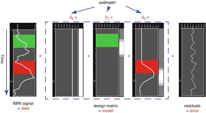
From the perspective of multiple regression analysis, the GLM aims to “explain” or “predict” the variation of a dependent variable in terms of a linear combination (weighted sum) of several reference functions. The dependent variable corresponds to the observed fMRI time course of a voxel, and the reference functions correspond to time courses of expected (idealized) fMRI responses for different conditions of the experimental paradigm. The reference functions are also called predictors, regressors, explanatory variables, covariates, or basis functions. A set of specified predictors forms the design matrix, also called the model. A predictor time course is typically obtained by convolution of a “boxcar” time course with a standard hemodynamic response function. A boxcar time course is usually defined by setting values to 1 at time points at which the modeled condition is defined (“on”) and 0 at all other time points.
Each predictor time course
x i gets an associated coefficient or
beta weight b i that quantifies the contribution of a predictor in explaining variance in the voxel time course
y. The voxel time course
y is modeled as the sum of the defined predictors, each multiplied with the associated beta weight
b. Since this linear combination will not perfectly explain the data due to noise fluctuations, an error value
e is added to the GLM system of equations with
n data points and
p predictors:
The y variable on the left side corresponds to the data, i.e., the measured time course of a single voxel. Time runs from top to bottom, i.e., y 1 is the measured value at time point 1, y 2 the measured value at time point 2, and so on. The voxel time course (left column) is “explained” by the terms on the right side of the equation. The first column on the right side corresponds to the first beta weight b 0. The corresponding predictor time course X 0 has a value of 1 for each time point and is, thus, also called “constant.” Since multiplication with 1 does not change the value of b 0, this predictor time course (X 0) does not explicitly appear in the equation. After estimation (see below), the value of b 0 typically represents the signal level of the baseline condition and is also called intercept. While its absolute value is not very informative in the context of fMRI data, it is important to include the constant predictor in a design matrix since it allows the other predictors to model small condition-related fluctuations as increases or decreases relative to the baseline signal level. The other predictors on the right side model the expected time courses of different conditions. For multifactorial designs, predictors may be defined that code combinations of condition levels allowing to estimate main and interaction effects. The beta weight of a predictor scales the associated predictor time course and reflects the unique contribution of that predictor in explaining the variance of the voxel time course. While the exact interpretation of beta values depends on the details of the design matrix, a large positive (negative) beta weight typically indicates that the voxel exhibits strong activation (deactivation) during the modeled experimental condition relative to baseline. All beta values together characterize a voxels “preference” for one or more experimental conditions. The last column in the system of equations contains error values, also called residuals, prediction errors, or noise. These error values quantify the deviation of the measured voxel time course from the predicted time course.
The GLM system of equations may be expressed elegantly using matrix notation. For this purpose, the voxel time course, the beta values, and the residuals are represented as vectors, and the set of predictors as a matrix:
Representing the indicated vectors and matrix with single letters, we obtain this simple form of the GLM system of equations:
In this notation, the matrix
X represents the
design matrix containing the predictor time courses as column vectors. The beta values now appear in a separate vector
b. The term
Xb indicates matrix-vector multiplication. Figure
1.2 shows a graphical representation of the GLM. Time courses of the signal, predictors, and residuals have been arranged in column form with time running from top to bottom as in the system of equations.
Given the data
y and the design matrix
X, the GLM fitting procedure has to find a set of beta values explaining the data as good as possible. The time course values

predicted by the model are obtained by the linear combination of the predictors:
A good fit would be achieved with beta values leading to predicted values

that are as close as possible to the measured values
y. By rearranging the system of equations, it is evident that a good prediction of the data implies small error values:
An intuitive idea would be to find those beta values minimizing the sum of error values. Since the error values contain both positive and negative values (and because of additional statistical considerations), the GLM procedure does not estimate beta values minimizing the sum of error values, but finds those beta values that
minimize the sum of squared error values:
The term
e′e is the vector notation for the sum of squares

. The apostrophe symbol denotes transposition of a vector (or matrix), i.e., a row vector version of
e is multiplied by a column vector version of
e resulting in the sum of squared values
e t . The optimal beta weights minimizing the squared error values (the “least squares estimates”) are obtained non-iteratively by the following equation:
The term in brackets contains a matrix-matrix multiplication of the transposed, X′, and non-transposed, X, design matrix. This term results in a square matrix with a number of rows and columns corresponding to the number of predictors. Each cell of the X′X matrix contains the scalar product of two predictor vectors. The scalar product is obtained by summing all products of corresponding entries of two vectors corresponding to the (non-mean normalized) calculation of covariance. This X′X matrix, thus, corresponds to the (non-mean normalized) predictor variance-covariance matrix.
The non-normalized variance-covariance matrix is inverted as denoted by the “−1” symbol. The resulting matrix (X′X)−1 plays an essential role not only for the calculation of beta values but also for testing the significance of contrasts (see below). The remaining term on the right side, X′y, evaluates to a vector containing as many elements as predictors. Each element of this vector is the scalar product (non-mean normalized covariance term) of a predictor time course with the observed voxel time course.
An important property of the least squares estimation method (following from the independence assumption of the errors, see below) is that the variance of the measured time course can be decomposed into the sum of the variance of the predicted values (model-related variance) and the variance of the residuals:
Since the variance of the voxel time course is fixed, minimizing the error variance by least squares corresponds to maximizing the variance of the values explained by a model. The square of the
multiple correlation coefficient R provides a measure of the proportion of the variance of the data which can be explained by a specified model:
The values of the multiple correlation coefficient vary between 0 (no variance explained) and 1 (all variance explained by the model). A coefficient of
R = 0.7, for example, corresponds to an explained variance of 49 % (0.7∙0.07). An alternative way to calculate the multiple correlation coefficient consists in computing a standard correlation coefficient between the predicted values and the observed values:

. This equation provides another view on the meaning of the multiple correlation coefficient quantifying the interrelationship (correlation) of the
combined set of optimally weighted predictor variables with the observed time course.
1.3.3.1 GLM Diagnostics
Note that if the design matrix (model) does not contain all relevant predictors, condition-related increases or decreases in the voxel time course will be explained by the error values instead of by the model. It is, therefore, important that the design matrix is constructed with all expected effects, which may also include reference functions not related to experimental conditions, for example, estimated motion parameters or drift predictors (if not removed during preprocessing, see Sect.
1.2.3). In case that all expected effects are properly modeled, the residuals should reflect only “pure” noise fluctuations. If some effects are not (correctly) modeled, a plot of the residuals may show low-frequency fluctuations instead of a stationary noisy time course. A visualization of the residuals (for selected voxels or regions of interest) is, thus, a good diagnostic to assess whether the design matrix has been specified properly.
1.3.3.2 GLM Significance Tests
The multiple correlation coefficient is an important measure of the “goodness of fit” of a GLM. In order to test whether a specified model significantly explains variance in a voxel time course, an
F statistic can be calculated for a
R value with
p−
1 degrees of freedom in the numerator and
n−
p degrees of freedom in the denominator:
An error probability value p can then be obtained for the calculated F statistics. A high F value (p value smaller than 0.05) indicates that the experimental conditions as a whole have a significant modulatory effect on the data time course (omnibus effect).
While the overall
F statistic may tell us whether the specified model significantly explains a voxel’s time course, it does not allow assessing which individual conditions differ significantly from each other. Comparisons between conditions can be formulated as
contrasts, which are linear combinations of beta values corresponding to specific null hypotheses. To test, for example, whether activation in a single condition 1 deviates significantly from baseline, the null hypothesis would be that there is no effect in the population, i.e., H
0 :
b 1 = 0. To test whether activation in condition 1 is significantly different from activation in condition 2, the null hypothesis would state that the beta values of the two conditions would not differ, H
0 : ⋅
b 1 =
b 2 or H
0 : (+1)
b 1 + (−1)
b 2 = 0. To test whether the mean of condition 1 and condition 2 differs from condition 3, the following contrast could be specified: H
0 : (
b 1 +
b 2)/2 =
b 3 or H
0 : (+1)
b 1 + (+1)
b 2 + (−2)b
3 = 0. The values used to multiply the respective beta values are often written as a
contrast vector c. In the latter example,
1 the contrast vector would be written as
c = [+1 + 1 − 2]. Using matrix notation, the linear combination defining a contrast can be written as the scalar product of contrast vector
c and beta vector
b. The null hypothesis can then be simply described as
c′
b = 0. For any number of predictors
k, such a contrast can be tested with the following
t statistic with
n−
p degrees of freedom:
The numerator of this equation contains the described scalar product of the contrast and beta vector. The denominator defines the standard error of c′b, i.e., the variability of the contrast estimate due solely to noise fluctuations. The standard error depends on the variance of the residuals Var(e) as well as on the design matrix X. With the known degrees of freedom, a t value for a specific contrast can be converted in an error probability value p using the incomplete beta function mentioned earlier. Note that the null hypotheses above were formulated as c′b = 0 implying a two–sided alternative hypothesis, i.e., Ha : c ′ b ≠ 0. For one-sided alternative hypotheses, e.g., Ha : b 1 > b 2, the obtained p value from a two-sided test can be simply divided by 2 to get the p value for the one-sided test. If this p value is smaller than 0.05 and if the t value is positive, the null hypothesis may be rejected.
1.3.3.3 Conjunction Analysis
Experimental research questions often lead to specific hypotheses, which can best be tested by the
conjunction of two or more contrasts. As an example, it might be interesting to test with contrast
c 1 whether condition 2 leads to significantly higher activity than condition 1
and with contrast
c 2 whether condition 3 leads to significantly higher activity than condition 2. This question could be tested with the following conjunction contrast:
c 1 ∧
c 2 = [−1 + 1 0] ∧ [0 − 1 + 1]. Note that a logical “and” operation is defined for Boolean values (true/false) but that
t values associated with individual contrasts can assume any real value. An appropriate way to implement a logical “and” operation for conjunctions of contrasts with continuous statistical values is to use a minimum operation, i.e., the significance level of the conjunction contrast is identical to the significance level of the contrast with the smallest
t value:
. For more details about conjunction testing, see Nichols et al. (
2006).
1.3.3.4 Event-Related Averaging
As mentioned earlier, event-related designs cannot only be used to
detect activation effects but also to
estimate the time course of task-related responses. Visualization of mean response profiles can be achieved by averaging all responses of the same condition across corresponding time points with respect to stimulus onset. Averaged (or even single trial) responses can be used to characterize the temporal dynamics of brain activity within and across brain areas by comparing estimated features such as response latency, duration, and amplitude (e.g., Kruggel and von Cramon
1999; Formisano and Goebel
2003). In more complex, temporally extended tasks, responses to subprocesses may be identified. In working memory paradigms, for example, encoding, delay and response phases of a trial may be separated. Note that event-related selective averaging works well only for slow event-related designs. In rapid event-related designs, responses from different conditions lead to substantial overlap, and event-related averages are often meaningless. In this case, deconvolution analysis is recommended (see below).
In order to avoid circularity, event-related averages should only be used descriptively if they are selected from significant clusters identified from a whole-brain statistical analysis of the same data. Even a merely descriptive analysis visualizing averaged condition responses is, however, helpful in order to ensure that significant effects are caused by “BOLD-like” response shapes and not by, e.g., signal drifts or measurement artifacts. If ROIs are determined using independent (localizer) data, event-related averages extracted from these regions in a subsequent (main) experiment can be statistically analyzed. For a more general discussion of ROI vs. whole-brain analyses, see Friston and Henson (
2006), Friston et al. (
2006), Saxe et al. (
2006), and Frost and Goebel (
2013).
1.3.4 Deconvolution Analysis
While standard design matrix construction (convolution of boxcar with two-gamma function) can be used to estimate condition amplitudes (beta values) in rapid event-related designs, results critically depend on the appropriateness of the assumed standard BOLD response shape: Due to variability in different brain areas within and across subjects, a static model of the response shape might lead to nonoptimal fits. Furthermore, the isolated responses to different conditions cannot be visualized due to overlap of condition responses over time. To model the shape of the hemodynamic response more flexibly, multiple basis functions (predictors) may be defined for each condition instead of one. Two often-used additional basis function sets are derivatives of the two-gamma function with respect to two of its parameters, delay and dispersion. If added to the design matrix for each condition, these basis functions allow capturing small variations in response latency and width of the response. Other sets of basis functions (i.e., gamma basis set, Fourier basis set) are much more flexible, but obtained results are often more difficult to interpret. Deconvolution analysis is a general approach to estimate condition-related response profiles using a flexible and interpretable set of basis functions. It can be easily implemented as a GLM by defining an appropriate design matrix that models each bin after stimulus onset by a separate condition predictor (delta or “stick” functions). This is also called a finite impulse response (FIR) model because it allows estimating any response shape evoked by a short stimulus (impulse). In order to capture the BOLD response for short events, about 20 s are typically modeled after stimulus onset. This would require, for each condition, 20 predictors in case of a TR of 1 s, or ten predictors in case of a TR of 2 s. Despite overlapping responses, fitting such a GLM “recovers” the underlying condition-specific response profiles in a series of beta values, which appear in plots as if event-related averages have been computed in a slow event-related design. Since each condition is modeled by a series of temporally shifted predictors, hypothesis tests can be performed that compare response amplitudes at different moments in time within and between conditions. Note, however, that deconvolution analysis assumes a linear time-invariant (LTI) system, i.e., it is assumed that overlapping responses can be modeled as the sum of individual responses. Furthermore, in order to uniquely estimate the large number of beta values from overlapping responses, variable ITIs must be used in the experimental design. The deconvolution model is very flexible allowing to capture any response shape. This implies that also non-BOLD-like time courses will be detected easily since the trial responses are not “filtered” by the ideal response shape as in conventional analysis.
 :
:  . Note that one would obtain in this example the same mean values in both conditions and, thus, the same difference in cases (a) and (b). Despite the fact that the means are identical in both cases, the difference in case b) seems to be more “trustworthy” than the difference in case (a) because the measured values exhibit less fluctuations, i.e., they vary less in case (b) than in case (a). Statistical data analysis goes beyond simple subtraction by taking into account the amount of variability of the measured data points. Statistical analysis essentially asks how likely it is to obtain a certain effect (e.g., difference of condition means) in a data sample if there is no effect at the population level, i.e., how likely it is that an observed sample effect is solely the result of noise fluctuations. This is formalized by the null hypothesis that states that there is no effect, i.e., no true difference between conditions in the population. In the case of comparing the two means μ1 and μ2, the null hypothesis can be formulated as H0: μ1 = μ2. Assuming the null hypothesis, it can be calculated how likely it is that an observed sample effect would have occurred simply by chance. This requires knowledge about the amount of noise fluctuations (and its distribution), which can be estimated from the data. By incorporating the number of data points and the variability of measurements, statistical data analysis allows to estimate the uncertainty of effects (e.g., of mean differences) in data samples. If an observed effect is large enough so that it is very unlikely that it has occurred simply by chance (e.g., the probability is less than p = 0.05), one rejects the null hypothesis and accepts the alternative hypothesis stating that there exists a true effect in the population. Note that the decision to accept or reject the null hypothesis is based on a probability value of p <0.05 that has been accepted by the scientific community. A statistical analysis, thus, does never prove the existence of an effect, it only suggests “to believe in an effect” if it is very unlikely that the observed effect would have occurred by chance. Note that a probability of p = 0.05 means that if we would repeat the experiment 100 times, we would accept the alternative hypothesis in about five cases even if there would be no real effect in the population. Since the chosen probability value thus reflects the likelihood of wrongly rejecting the null hypothesis, it is also called error probability. The error probability is also referred to as the significance level and denoted with the Greek letter α. If one would know that there is no effect in the population but one would incorrectly reject the null hypothesis in a particular data sample, a “false-positive” decision would be made (type 1 error). Since a false-positive error depends on the chosen error probability, it is also referred to as alpha error. If one would know that there is a true effect in the population but one would fail to reject the null hypothesis in a sample, a “false-negative” decision would be made, i.e., one would miss a true effect (type 2 error or beta error).
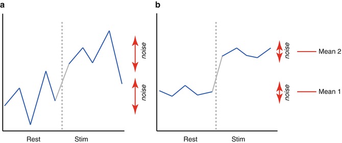

![$$ \left[\begin{array}{c}{y}_1\\ {}\vdots \\ {}\vdots \\ {}{y}_n\end{array}\right]=\left[\begin{array}{ccccc}1& {X}_{11}& \cdots & \cdots & {X}_{1p}\\ {}\vdots & \vdots & \vdots & \vdots & \vdots \\ {}\vdots & \vdots & \vdots & \vdots & \vdots \\ {}1& {X}_{n1}& \cdots & \cdots & {X}_{np}\end{array}\right]\left[\begin{array}{c}{b}_0\\ {}{b}_1\\ {}\vdots \\ {}{b}_p\end{array}\right]+\left[\begin{array}{c}{e}_1\\ {}{e}_2\\ {}\vdots \\ {}{e}_n\end{array}\right] $$](/wp-content/uploads/2016/03/A214842_1_En_1_Chapter_Equd.gif)


![$$ E\left[{\varepsilon}_i\right]=0 $$](/wp-content/uploads/2016/03/A214842_1_En_1_Chapter_Equn.gif)
![$$ Var\left[{\varepsilon}_i\right]={\sigma}^2 $$](/wp-content/uploads/2016/03/A214842_1_En_1_Chapter_Equo.gif)