(3.1)
where F is some nonlinear function describing the neurophysiological influences exerted by inputs u and the activity in all brain regions on the evolution of the neuronal states. A bilinear approximation provides a natural and useful re-parameterisation in terms of coupling parameters.
(3.2)
The (effective) connectivity matrix A represents the first-order coupling among the regions in the absence of inputs. This can be thought of as the endogenous coupling in the absence of experimental perturbations. Note that the state, which is perturbed, depends on the experimental design (e.g. baseline or control state), and therefore, the endogenous coupling is specific to each experiment. The matrices B (j) are the change in endogenous coupling induced by the jth input (Fig. 3.1 Finally, the matrix C encodes the exogenous (driving) influences of inputs on neuronal activity. The parameters θ c = {A, B (j), C} are the coupling parameter matrices we wish to estimate and define the functional architecture and interactions among brain regions at a neuronal level. Note that the units of coupling are per unit time (Hz) and therefore correspond to rates. Because we are in a dynamic setting, a strong connection means an influence that is expressed quickly or with a small time constant. It is useful to appreciate this when interpreting estimates and thresholds quantitatively.
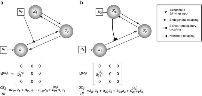
Fig. 3.1
This diagram illustrates two types of ‘modulatory’ effects – the bilinear (a) and the nonlinear (b) modulations. The target of modulation is made over the z 1-to-z 2 coupling. The difference between the neuronal state equations for z 2 is made explicit in the respective panels (see the last term). Specifically, the bilinear model allows an exogenous experimental manipulation (u 2) to induce connectivity change. The nonlinear model, on the other hand, manifests the neuronal origin (z 3, as now encodes u 2) of the modulatory effect
The neuronal activity in each region causes changes in volume and deoxyhaemoglobin which engender the observed BOLD response y as described below. The ensuing haemodynamic component of the model is specific to BOLD-fMRI and would be replaced by appropriate forward models for other imaging modalities, such as EEG or MEG.
The neuronal dynamics in Eq. (3.2) operate around a stable fixed point z = 0 (strictly speaking, this will only be the case for certain ranges of parameter values – see Friston et al. 2003). This means that, in the absence of exogenous perturbations, the neuronal activity and consequently the fMRI activity will be zero. Briefly, a neuronal state in DCM predicts nothing but a flat line if it is not experimentally perturbed, directly or indirectly (but see Li et al. 2011a). This is because DCM for fMRI is based on a dynamic system with a fixed point attractor.
3.2.3 Nonlinear DCM
Nonlinear DCM (Stephan et al. 2008) introduces a parametric matrix D that allows neuronal activity in one region to change the connectivity between other regions (Fig. 3.1 This is in contrast to bilinear dynamics (Eq. 3.2) in which, perhaps unrealistically, effective connectivity can be changed via ‘modulatory inputs’.
(3.3)
The motivation for this extension is to address ‘neuronal gain control’ between two neuronal states that are gated by other states (Stephan et al. 2008). The approach also models the neuronal origin of modulatory influences such as ‘short-term synaptic plasticity’ (Stephan et al. 2008). Applications based on nonlinear DCM can be found in den Ouden et al. (2010) and Table 3.1 (Desseilles et al. 2011; Neufang et al. 2011).
Table 3.1
List of DCM applications in psychiatric neuroimaging studies (shown in publication year-alphabetical order)
Study | Patientcondition | Activationparadigm | Number of participants | N | M | Inference type | Findings |
|---|---|---|---|---|---|---|---|
Almeidaet al. (2009) | Bipolar disorder, major depressive disorder | Emotional regulation (labelling happy vs. sad faces) | 15 BD, 16 MDD,16 controls | 2/BL | 1 | Parameter (classical) | Hemispheric and directional asymmetry in OMPFC-amygdala connectivity differentiates between BD and MDD abnormality |
Schlösseret al. (2010) | Obsessive-compulsive disorder | Stroop task (colour-word congruency) | 21 patients,21 controls | 6/BL | 5 | Model (RFX-BMS), parameter (classical) | OCD predominant fronto-cingulate connectivity enhancement subject to incongruent Stroop modulation |
Almeidaet al. (2011) | Major depressive disorder | Automatic attentional control of emotion | 19 patients,19 controls | 3/BL | 1 | Parameter (classical) | Characteristic cortico-amygdala connectivity alterations to happy and fearful stimuli in female MDD |
Bányaiet al. (2011) | Schizophrenia | Associative learning (object-location) | 11 patients,11 controls | 5/BL | 24 | Model (RFX-BMS), parameter (classical, BPA) | Information processing network in schizophrenia is different from that of controls. No specific impaired pathway can be identified |
Reduced fronto-hippocampal and hippocampo-IT connectivity in patients | |||||||
Desseilleset al. (2011) | Major depressive disorder | Visual detection task | 14 patients,14 controls | 3/NL | 10 (2 families) | Family, model (RFX-BMS), parameter (BPA) | Control: high attentional load was associated with negative IPS-V4 modulation |
Patient: attention levels exerted modulations on IPS | |||||||
van Leeuwenet al. (2011) | Synaesthesia | Colour-controlled grapheme viewing | 19 synaesthetes (‘projectors’ vs. ‘associators’) | 3/BL | 2 | Model (RFX-BMS), parameter (BPA) | Synaesthetic V4 cross-activation induced bottom-up and top-down pathways for projector and associator synaesthetes, respectively |
Li et al.(2011b) | None included | TMS-triggered vs. visually cued thumb movement | 0 patient, 25 (M1)/21 (PFC) controls | 4(M1), 3(PFC)/BL | 4 (M1), 3 (PFC) | Model (FFX-BMS), parameter (average) | LTG and VPA reduced motor circuitry connectivity, whereas VPA enhanced prefrontal circuitry connectivity |
Neufanget al. (2011) | Prodromal Alzheimer’s disease | Attentional network task | 15 patients,16 controls | 4/NL | 4 | Model (RFX-BMS), parameter (classical) | Reduced frontoparietal connectivity corresponded to regional grey matter volume and attentional control |
Desernoet al. (2012) | Schizophrenia | Numeric n-back (2-back vs. 0-back) | 41 patients,42 controls | 3/BL | 48 (3 families) | Family, model (RFX-BMS), parameter (BMA, classical) | Identification of disrupted WM-dependent corticocortical dynamics contributing DLPFC inefficiency and cognitive deficits in schizophrenia |
Diwadkaret al. (2012) | None included | Emotional processing | 19 schizophrenic patient offspring,24 controls | 5/BL | 136 | Model (RFX-/FFX-BMS), parameter (classical) | High-risk schizophrenic group exhibited declined visual driving, declined frontolimbic intrinsic coupling and increased inhibitory frontolimbic modulation by negative valence |
Passamontiet al. (2012) | None included | Emotional regulation with placebo-controlled ATD | 0 patient,19 controls | 3/BL | 49 (7 families, 3 ‘meta-families’) | Family | ATD procedure reduced emotional processing within PFC-amygdala pathways |
3.2.4 Haemodynamics
Neuronal activity is linked to fMRI signals via an extended Balloon model (Buxton et al. 1998, 2004) and BOLD signal model (Stephan et al. 2007b). The haemodynamic model specifies how changes in neuronal activity give rise to changes in blood oxygenation that is measured with fMRI. For each region i, neuronal activities are translated into BOLD signals via the interactions between the neuronal state z i and haemodynamic state variables: the vasodilatory signal, the flow induced, changes in volume, and changes in deoxyhaemoglobin. The observed BOLD signals are produced by a nonlinear model that integrates over the states, y = g(v, q), where the evolution of v and q over time depends on self-regulatory feedback as well as s and f (cf. to Fig. 3 in Friston et al. 2003). The equations for the haemodynamics are described in detail elsewhere (Grubb et al. 1974; Buxton et al. 1998; Mandeville et al. 1999; Friston et al. 2000).
3.2.5 Priors
Two classes of prior densities are used in DCM; they are placed over coupling and haemodynamic parameters θ = {A, B, C, θ h}. DCM uses ‘shrinkage priors’ over coupling parameters. These are zero-mean Gaussian priors with a variance that is chosen to reflect realistic ranges in effective connectivity seen in fMRI studies. These shrinkage priors move the posterior estimates towards zero, especially when the likelihood has a less precise distribution. For example, the posterior expectation will ‘shrink’ to its prior expectation given a likelihood with a very large variance. However, a likelihood that has high precision (inverse variance) enforces the posterior to deviate from zero. Prior variances can also be chosen to reflect anatomical knowledge, for example, probabilistic tractography (Stephan et al. 2009). Haemodynamic priors in DCM reflect empirical knowledge about blood flow and oxygenation dynamics in the brain (Buxton et al. 1998, 2004). The prior densities of the five haemodynamic parameters θ h = {κ, γ, τ, α, ρ} that mediate the interactions among these states are set based on empirical measures (see Eq. (3.3) and Table 3.1 in Friston et al. 2003). These priors have since been updated in light of more recent data (Penny 2012).
3.2.6 Model Fitting
DCMs are fitted to data using the Variational Laplace (VL) algorithm described in (Friston et al. 2007). This is an iterative algorithm which approximates the posterior distribution over parameters with a Gaussian distribution. The parameters of this distribution are updated so as to minimise the distance between the approximate and true posterior, in the sense of Kullback-Leibler divergence – a distance measure between probability densities (MacKay 2003). The VL algorithm provides estimates of two quantities. The first is the posterior density over model parameters p(θ|m, y) that can be used to make inferences about model parameters θ. The second is the probability of the data given the model, otherwise known as the model evidence p(y|m).
3.2.7 Parameter Inference for Single Models
Inferences about DCM parameters – based on single models – require strong assumptions about network structure based on well-established neurophysiological, cognitive or anatomical evidence. For instance, Almeida and colleagues demonstrated that the uncinate fasciculus, which provides orbitofronto-amygdala circuitry, mediates emotional regulation and is abnormal in bipolar disorder patients, in terms of fractional anisotropy (Almeida et al. 2009). Both single-model studies reviewed here (Almeida et al. 2009, 2011) used a fully connected model to allow all possible coupling parameters to be estimated. They found that left-sided, top-down orbitomedial prefrontal cortex (OMPFC) to amygdala and right-sided bottom-up amygdala to OMPFC distinguished bipolar from major depression.
3.2.8 Model Evidence
In general, model evidence is not straightforward to compute, since this computation involves integrating out the dependence on model parameters:
(3.4)
Therefore, an approximation to the model evidence is required. DCM uses the free-energy approximation to the model evidence provided by the VL algorithm. The model evidence, and the VL approximation to it, naturally embodies the accuracy-complexity trade-off that is the hallmark of a good model (Pitt and Myung 2002


Related posts:

Stay updated, free articles. Join our Telegram channel
Full access? Get Clinical Tree
