Fig. 1
Some application areas of image processing that essentially rely on image motion analysis. Left: scene analysis (depth, independently moving objects) with a camera mounted in a car. Center: flow analysis in remote sensing. Right: measuring turbulent flows by particle image velocimetry
Due to this independency, optical flow algorithms provide a key component for numerous approaches to applications across different fields. Major examples include motion compensation for video compression, structure from motion to estimate 3-D scene layouts from image sequences, visual odometry, and incremental construction of mappings of the environment by autonomous systems, estimating vascular wall shear stress from blood flow image sequences for biomedical diagnosis, to name just a few.
This chapter aims at providing a concise and up-to-date account of mathematical models of optical flow estimation. Basic principles are presented along with various prior models. Application-specific aspects are only taken into account at a general level of mathematical modeling (e.g., geometric or physical prior knowledge). Model properties favoring a particular direction of modeling are highlighted, while keeping an eye on common aspects and open problems. Conforming to the editor’s guidelines, references to the literature are confined to a – subjectively defined – essential minimum.
Organization
Section 2 introduces a dichotomy of models used to present both essential differences and common aspects. These classes of models are presented in Sects. 3 and 4. The former class comprises those algorithms that perform best on current benchmark datasets. The latter class becomes increasingly more important in connection with motion analysis of novel, challenging classes of image sequences and videos. While both classes merely provide different viewpoints on the same subject – optical flow estimation and image motion analysis – distinguishing them facilitates the presentation of various facets of relevant mathematical models in current research. Further relationships, unifying aspects together with some major open problems and research directions, are addressed in Sect. 5.
2 Basic Aspects
Invariance, Correspondence Problem
Image motion computation amounts to define some notion of invariance and the recognition in subsequent time frames of corresponding objects, defined by local prominent image structure in terms of a feature mapping g(x) whose values are assumed to be conserved during motion. As Fig. 2, left panel, illustrates, invariance only holds approximately due to the imaging process and changes of viewpoint and illumination. Consequently, some distance function

has to be used in order to compute an optimal assignment
![$$\displaystyle{ \{g(x^{i},t)\}_{ i\in [m]} \rightarrow \{ g(x^{j},t +\delta t)\}_{ j\in [n]}. }$$](/wp-content/uploads/2016/04/A183156_2_En_38_Chapter_Equ2.gif)
A vast literature exists on definitions of feature mappings g(x, t), distance functions, and their empirical evaluation in connection with image motion. Possible definitions include


(1)
![$$\displaystyle{ \{g(x^{i},t)\}_{ i\in [m]} \rightarrow \{ g(x^{j},t +\delta t)\}_{ j\in [n]}. }$$](/wp-content/uploads/2016/04/A183156_2_En_38_Chapter_Equ2.gif)
(2)
Image gray value or color,
Gray value or color gradient,
Censor voting, [5], local patches or feature groupings,

Fig. 2
Left: image motion can only be computed by recognizing objects as the same in subsequent time frames, based on some notion of equivalence (invariance) and some distance function. In low-level vision, “object” means some prominent local image structure in terms a feature mapping  . The correspondence problem amounts to compute a corresponding assignment
 ![$$\{g(x^{i},t)\}_{i\in [m]} \rightarrow \{ g(x^{j},t +\delta t)\}_{j\in [n]}$$](/wp-content/uploads/2016/04/A183156_2_En_38_Chapter_IEq2.gif) . The corresponding objective defines the data term of a variational approach. Right: differential approaches to image motion computation are based on smooth feature mappings g(x, t) and aim at solving the assignment problem
. The corresponding objective defines the data term of a variational approach. Right: differential approaches to image motion computation are based on smooth feature mappings g(x, t) and aim at solving the assignment problem  . The figure illustrates the basic case of a scalar-valued signal g(x, t) translating with constant speed u and the estimate (14) based on the differential motion approach, as discussed in section “Assignment Approach, Differential Motion Approach”
 . The correspondence problem amounts to compute a corresponding assignment
 ![$$\{g(x^{i},t)\}_{i\in [m]} \rightarrow \{ g(x^{j},t +\delta t)\}_{j\in [n]}$$](/wp-content/uploads/2016/04/A183156_2_En_38_Chapter_IEq2.gif) . The corresponding objective defines the data term of a variational approach. Right: differential approaches to image motion computation are based on smooth feature mappings g(x, t) and aim at solving the assignment problem
. The corresponding objective defines the data term of a variational approach. Right: differential approaches to image motion computation are based on smooth feature mappings g(x, t) and aim at solving the assignment problem  . The figure illustrates the basic case of a scalar-valued signal g(x, t) translating with constant speed u and the estimate (14) based on the differential motion approach, as discussed in section “Assignment Approach, Differential Motion Approach”
together with a corresponding invariance assumption, i.e., that g(x, t) is conserved during motion (cf. Fig. 2, left panel). Figure 3 illustrates the most basic approaches used in the literature. Recent examples adopting a more geometric viewpoint on feature descriptors and studying statistical principles of patch similarity include [6, 7].
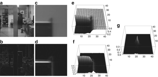

Fig. 3
(a) Lab scene (©CMU image database) and (b) gradient magnitude that provides the basis for a range of feature mappings g(x, t). The image section indicated in (a) is shown in (c), and (d) shows the same section extracted from (b). Panels (e) and (f) illustrate these sections as surface plots. Panel (g) shows a feature map responding to crossing gray-value edges. (c), (d), and (g) correspond to the most basic examples of feature mappings g(x, t) used in the literature to compute image motion, based on a corresponding invariance assumption (cf. Fig. 2, left panel) that is plausible for video frame rates
For further reference, some basic distance functions  are introduced below that are commonly applied in connection with feature mappings g(x) and partly parametrized by λ > 0 and
  . For closely related functions and the nomenclature in computer vision, see, e.g., [8].


![$$\displaystyle\begin{array}{rcl} \begin{array}{l@{\qquad \qquad \qquad }r} \rho _{1,\varepsilon }(z):=\sum _{i\in [p]}\rho _{2,\varepsilon }(z_{i})\qquad \qquad \qquad &\text{smoothed}\;\ell^{1}\;\text{distance},\end{array} & &{}\end{array}$$](/wp-content/uploads/2016/04/A183156_2_En_38_Chapter_Equ7.gif)


 are introduced below that are commonly applied in connection with feature mappings g(x) and partly parametrized by λ > 0 and
  . For closely related functions and the nomenclature in computer vision, see, e.g., [8].
(3a)

(3b)

(3c)

(3d)
![$$\displaystyle\begin{array}{rcl} \begin{array}{l@{\qquad \qquad \qquad }r} \rho _{1,\varepsilon }(z):=\sum _{i\in [p]}\rho _{2,\varepsilon }(z_{i})\qquad \qquad \qquad &\text{smoothed}\;\ell^{1}\;\text{distance},\end{array} & &{}\end{array}$$](/wp-content/uploads/2016/04/A183156_2_En_38_Chapter_Equ7.gif)
(3e)

(3f)

(3g)
Figure 4 illustrates these convex and non-convex distance functions. Functions  and
and  constitute specific instances of the general smoothing principle to replace a lower semicontinuous, positively homogeneous, and sublinear function ρ(z) by a smooth proper convex function
  , with
  (cf., e.g., [9]). Function
  utilizes the log-exponential function [10, Ex. 1.30] to uniformly approximate
  as
as  .
.
 and
and  constitute specific instances of the general smoothing principle to replace a lower semicontinuous, positively homogeneous, and sublinear function ρ(z) by a smooth proper convex function
  , with
  (cf., e.g., [9]). Function
  utilizes the log-exponential function [10, Ex. 1.30] to uniformly approximate
  as
as  .
.Assignment Approach, Differential Motion Approach
Definitions
Two basic approaches to image motion computation can be distinguished.
Assignment Approach, Assignment Field
This approach aims to determine an assignment of finite sets of spatially discrete features in subsequent frames of a given image sequence (Fig. 2, left panel). The vector field

representing the assignment in Eq. (2), is called assignment field. This approach conforms to the basic fact that image sequences f(x, t), (x, t) ∈ Ω× [0, T] are recorded by sampling frames

along the time axis.

(4)

(5)
Assignment approaches to image motion will be considered in Sect. 4.
Differential Motion Approach, Optical Flow
Starting point of this approach is the invariance assumption (section “Invariance, Correspondence Problem”) that observed values of some feature map g(x, t) are conserved during motion,

Evaluating this condition yields information about the trajectory x(t) that represents the motion path of a particular feature value  . The corresponding vector field

is called motion field whose geometric origin will be described in section “Two-View Geometry, Assignment and Motion Fields.” Estimates

of the motion field based on some observed time-dependent feature map g(x, t) are called optical flow fields.

(6)
 . The corresponding vector field
(7)

(8)
Differential motion approaches will be considered in Sect. 3.
Common Aspects and Differences
The assignment approach and the differential approach to image motion are closely related. In fact, for small temporal sampling intervals,

one may expect that the optical flow field multiplied by δ t, u(x, t) ⋅ δ t, closely approximates the corresponding assignment field. The same symbol u is therefore used in (4) and (8) to denote the respective vector fields.

(9)
A conceptual difference between both approaches is that the ansatz (6) entails the assumption of a spatially differentiable feature mapping g(x, t), whereas the assignment approach requires prior decisions done at a preprocessing stage that localize the feature sets (2) to be assigned. The need for additional processing in the latter case contrasts with the limited applicability of the differential approach: The highest spatial frequency limits the speed of image motion  that can be estimated reliably:

The subsequent section details this bound in the most simple setting for a specific but common filter choice for estimating partial derivatives ∂ i g.
 that can be estimated reliably:
(10)
Differential Motion Estimation: Case Study (1D)
Consider a scalar signal g(x, t) = f(x, t) moving at constant speed (cf. Fig. 2, right panel),

Note that the two-dimensional function g(x, t) is a very special one generated by motion. Using the shorthands

g(x, t) corresponds to the translated one-dimensional signal

due to the assumption  .
.

(11)

(12)

(13)
 .
.Evaluating (6) at t = 0, x = x(0) yields

Application and validity of this equation in practice depends on two further aspects: Only sampled values of g(x, t) are given, and the right-hand side has to be computed numerically. Both aspects are discussed next in turn.

(14)
1.
In practice, samples are observed

with the sampling interval scaled to 1 without loss of generality. The Nyquist-Shannon sampling theorem imposes the constraint

where

denotes the Fourier transform of g(x, t). Trusting in the sensor, it may be savely assumed that  . But what about the second coordinate t generated by motion? Does it obey (16) such that the observed samples (15) truly represent the one-dimensional video signal g(x, t)?

(15)

(16)

(17)
 . But what about the second coordinate t generated by motion? Does it obey (16) such that the observed samples (15) truly represent the one-dimensional video signal g(x, t)?
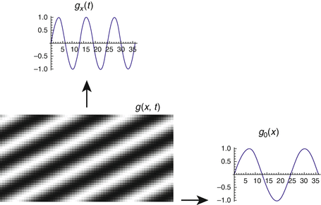
To answer this question, consider the specific case ![$$g_{0}(x) =\sin (\omega _{x}x),\,\omega _{x} \in [0,\pi ]$$](/wp-content/uploads/2016/04/A183156_2_En_38_Chapter_IEq17.gif) – see Fig. 5. Equation (13) yields
– see Fig. 5. Equation (13) yields  . Condition (15) then requires that, for every location x, the one-dimensional time signal g x (t): = g(x, t) satisfies
  . Applying this to the example yields

and hence the condition

It implies that Eq. (14) is only valid if, depending on the spatial frequency ω x , the velocity u is sufficiently small.
![$$g_{0}(x) =\sin (\omega _{x}x),\,\omega _{x} \in [0,\pi ]$$](/wp-content/uploads/2016/04/A183156_2_En_38_Chapter_IEq17.gif) – see Fig. 5. Equation (13) yields
– see Fig. 5. Equation (13) yields  . Condition (15) then requires that, for every location x, the one-dimensional time signal g x (t): = g(x, t) satisfies
  . Applying this to the example yields
(18)

(19)
This reasoning and the conclusion apply to general functions  in the form of (10), which additionally takes into account the effect of derivative estimation, discussed next.
 in the form of (10), which additionally takes into account the effect of derivative estimation, discussed next.
2.
Condition (19) has to be further restricted in practice, depending on how the partial derivatives of the r.h.s. of Eq. (14) are numerically computed using the observed samples (15). The Fourier transform

generally shows that taking partial derivatives of order | α | of  , corresponds to high-pass filtering that amplifies noise. If g(x, t) is vector valued, then the present discussion applies to the computation of partial derivatives ∂ α g i of any component g i (x, t), i ∈ [p].

(20)
 , corresponds to high-pass filtering that amplifies noise. If g(x, t) is vector valued, then the present discussion applies to the computation of partial derivatives ∂ α g i of any component g i (x, t), i ∈ [p].
To limit the influence of noise, partial derivatives of the low-pass filtered feature mapping g are computed. This removes noise and smoothes the signal, and subsequent computation of partial derivatives becomes more accurate. Writing  , instead of
  , to simplify the following formulas, low-pass filtering of g with the impulse response h(x) means the convolution

whose Fourier transform corresponds to the multiplication of the respective Fourier transforms. Applying (20) yields

Thus, computing the partial derivative of the filtered function g h can be computed by convolving g with the partial derivative of the impulse response ∂ α h. As a result, the approximation of the partial derivative of g reads

The most common choice of h is the isotropic Gaussian low-pass filter
![$$\displaystyle{ h_{\sigma }(x):= \frac{1} {(2\pi \sigma ^{2})^{d/2}}\exp \Big(-\frac{\|x\|^{2}} {2\sigma ^{2}} \Big) =\prod _{i\in [d]}h_{\sigma }(x_{i}),\qquad \sigma > 0 }$$
” src=”/wp-content/uploads/2016/04/A183156_2_En_38_Chapter_Equ30.gif”></DIV></DIV><br />
<DIV class=EquationNumber>(24)</DIV></DIV>that factorizes (called <SPAN class=EmphasisTypeItalic>separable filter</SPAN>) and therefore can be implemented efficiently. The corresponding filters <SPAN id=IEq24 class=InlineEquation><IMG alt=](/wp-content/uploads/2016/04/A183156_2_En_38_Chapter_IEq24.gif) are called Derivative-of-Gaussian (DoG) filters.
are called Derivative-of-Gaussian (DoG) filters.
 , instead of
  , to simplify the following formulas, low-pass filtering of g with the impulse response h(x) means the convolution
(21)

(22)

(23)
![$$\displaystyle{ h_{\sigma }(x):= \frac{1} {(2\pi \sigma ^{2})^{d/2}}\exp \Big(-\frac{\|x\|^{2}} {2\sigma ^{2}} \Big) =\prod _{i\in [d]}h_{\sigma }(x_{i}),\qquad \sigma > 0 }$$
” src=”/wp-content/uploads/2016/04/A183156_2_En_38_Chapter_Equ30.gif”></DIV></DIV><br />
<DIV class=EquationNumber>(24)</DIV></DIV>that factorizes (called <SPAN class=EmphasisTypeItalic>separable filter</SPAN>) and therefore can be implemented efficiently. The corresponding filters <SPAN id=IEq24 class=InlineEquation><IMG alt=](/wp-content/uploads/2016/04/A183156_2_En_38_Chapter_IEq24.gif) are called Derivative-of-Gaussian (DoG) filters.
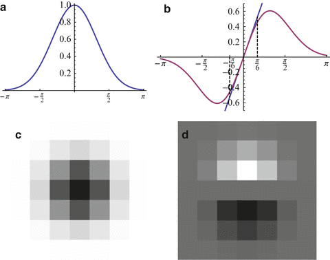
are called Derivative-of-Gaussian (DoG) filters. To examine its effect, it suffices to consider any coordinate due to factorization, that is, the one-dimensional case. Figure 6 illustrates that values σ ≥ 1 lead to filters that are sufficiently band limited so as to conform to the sampling theorem. The price to pay for effective noise suppression however is a more restricted range ![$$\text{supp}\vert \mathcal{F}\big(g(x,t)\big)\vert = [0,\omega _{x,\max }],\,\omega _{x,\max } \ll \pi$$](/wp-content/uploads/2016/04/A183156_2_En_38_Chapter_IEq25.gif) that observed image sequence functions have to satisfy, so as to enable accurate computation of partial derivatives and in turn accurate motion estimates based on the differential approach. Figure 5 further details and illustrates this crucial fact.
that observed image sequence functions have to satisfy, so as to enable accurate computation of partial derivatives and in turn accurate motion estimates based on the differential approach. Figure 5 further details and illustrates this crucial fact.
![$$\text{supp}\vert \mathcal{F}\big(g(x,t)\big)\vert = [0,\omega _{x,\max }],\,\omega _{x,\max } \ll \pi$$](/wp-content/uploads/2016/04/A183156_2_En_38_Chapter_IEq25.gif) that observed image sequence functions have to satisfy, so as to enable accurate computation of partial derivatives and in turn accurate motion estimates based on the differential approach. Figure 5 further details and illustrates this crucial fact.
that observed image sequence functions have to satisfy, so as to enable accurate computation of partial derivatives and in turn accurate motion estimates based on the differential approach. Figure 5 further details and illustrates this crucial fact. 
Fig. 5
A sinusoid g 0(x) with angular frequency ω x = π∕12, translating with velocity u = 2, generates the function g(x, t). The angular frequency of the signal g x (t) observed at a fixed position x equals | ω t | = u ⋅ ω x = π∕6 due to (18). It meets the upper bound further discussed in connection with Fig. 6 that enables accurate numerical computation of the partial derivatives of g(x, t)

Fig. 6
(a) Fourier transform  of the Gaussian low pass (24), σ = 1. For values σ ≥ 1, it satisfies the sampling condition
  sufficiently accurate. (b) The Fourier transform of the Derivative-of-Gaussian (DoG) filter
  illustrates that for | ω | ≤ π∕6 (partial) derivatives are accurately computed, while noise is suppressed at higher angular frequencies. (c), (d) The impulse responses h σ (x, t) and ∂ t h σ (x, t) up to size | x | , | t | ≤ 2. Application of the latter filter together with ∂ x h σ (x, t) to the function g(x, t) discussed in connection with Fig. 5 and evaluation of Eq. (14) yield the estimate u = 2. 02469 at all locations (x, t) where ∂ x g(x, t) ≠ 0
 of the Gaussian low pass (24), σ = 1. For values σ ≥ 1, it satisfies the sampling condition
  sufficiently accurate. (b) The Fourier transform of the Derivative-of-Gaussian (DoG) filter
  illustrates that for | ω | ≤ π∕6 (partial) derivatives are accurately computed, while noise is suppressed at higher angular frequencies. (c), (d) The impulse responses h σ (x, t) and ∂ t h σ (x, t) up to size | x | , | t | ≤ 2. Application of the latter filter together with ∂ x h σ (x, t) to the function g(x, t) discussed in connection with Fig. 5 and evaluation of Eq. (14) yield the estimate u = 2. 02469 at all locations (x, t) where ∂ x g(x, t) ≠ 0
Assignment or Differential Approach?
For image sequence functions g(x, t) satisfying the assumptions necessary to evaluate the key equation (6), the differential motion approach is more convenient. Accordingly, much work has been devoted to this line of research up to now. In particular, sophisticated multiscale representations of g(x, t) enable to estimate larger velocities of image motion using smoothed feature mapping g (cf. section “Multiscale”). As a consequence, differential approaches rank top at corresponding benchmark evaluations conforming to the underlying assumptions [11], and efficient implementations are feasible [12, 13].
On the other hand, the inherent limitations of the differential approach discussed above become increasingly more important in current applications, like optical flow computation for traffic scenes taken from a moving car at high speed. Figure 1, right panel, shows another challenging scenario where the spectral properties  of the image sequence function and the velocity fields to be estimated render application of the differential approach difficult, if not impossible. In such cases, the assignment approach is the method of choice.
 of the image sequence function and the velocity fields to be estimated render application of the differential approach difficult, if not impossible. In such cases, the assignment approach is the method of choice.
Combining both approaches in a complementary way seems most promising: Robust assignments enable to cope with fast image motions and a differential approach turns these estimates into spatially dense vector fields. This point is taken up in section “Unifying Aspects: Assignment by Optimal Transport.”
Basic Difficulties of Motion Estimation
This section concludes with a list of some basic aspects to be addressed by any approach to image motion computation:
(i)
Definition of a feature mapping g assumed to be conserved during motion (section “Invariance, Correspondence Problem”).
(ii)
Coping with lack of invariance of g, change of appearance due to varying viewpoint and illumination (sections “Handling Violation of the Constancy Assumption” and “Patch Features”).
(iii)
Spatial sparsity of distinctive features (section “Regularization”).
(iv)
Coping with ambiguity of locally optimal feature matches (section “Assignment by Displacement Labeling”).
(v)
Occlusion and disocclusion of features.
(vi)
Consistent integration of available prior knowledge, regularization of motion field estimation (sections “Geometrical Prior Knowledge” and “Physical Prior Knowledge”).
(vii)
Runtime requirements (section “Algorithms”).
Two-View Geometry, Assignment and Motion Fields
This section collects few basic relationships related to the Euclidean motion of a perspective camera relative to a 3-D scene that induces both the assignment field and the motion field on the image plane, as defined in section “Definitions” by (4) and (7). Figures 7 and 12 illustrate these relationships. References [14, 15] provide comprehensive expositions.
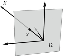

Fig. 7
The basic pinhole model of the mathematically ideal camera. Scene points X are mapped to image points x by perspective projection
It is pointed out once more that assignment and motion fields are purely geometrical concepts. The explicit expressions (43) and (53b) illustrate how discontinuities of these fields correspond to discontinuities of depth or to motion boundaries that separate regions in the image plane of scene objects (or the background) with different motions relative to the observing camera. Estimates of either field will be called optical flow, to be discussed in subsequent sections.
Two-View Geometry
Scene and corresponding image points are denoted by  and
and  , respectively. Both are incident with the line
  , through the origin. Such lines are points of the projective plane denoted by
  . The components of y are called homogeneous coordinates of the image point x, whereas x and X are the inhomogeneous coordinates of image and scene points, respectively. Note that y stands for any representative point on the ray connecting x and X. In other words, when using homogeneous coordinates, scale factors do not matter. This equivalence is denoted by

Figure 7 depicts the mathematical model of a pinhole camera with the image plane located at X 3 = 1. Perspective projection corresponding to this model connects homogeneous and inhomogeneous coordinates by

A particular representative y with unknown depth y 3 = X 3 equals the scene point X. This reflects the fact that scale cannot be inferred from a single image. The 3-D space  corresponds to the affine chart
  of the manifold
  .
.
 and
and  , respectively. Both are incident with the line
  , through the origin. Such lines are points of the projective plane denoted by
  . The components of y are called homogeneous coordinates of the image point x, whereas x and X are the inhomogeneous coordinates of image and scene points, respectively. Note that y stands for any representative point on the ray connecting x and X. In other words, when using homogeneous coordinates, scale factors do not matter. This equivalence is denoted by
(25)

(26)
 corresponds to the affine chart
  of the manifold
  .
.Similar to representing an image point x by homogeneous coordinates y, it is common to represent scene points  by homogeneous coordinates
  , in order to linearize transformations of 3-D space. The connection analogous to (26) is

Rigid (Euclidean) transformations are denoted by  with translation vector h and proper rotation matrix R ∈ SO(3) characterized by R ⊤ R = I, detR = +1. Application of the transformation to a scene point X and some representative Y reads

whereas the inverse transformation  yields

The nonlinear operation (26), entirely rewritten with homogeneous coordinates, takes the linear form

with the projection matrix P and external or motion parameters {h, R}. In practice, additional internal parameters characterizing real cameras to the first order of approximation are taken into account in terms of a camera matrix K and the corresponding modification of (30),

As a consequence, the transition to normalized (calibrated) coordinates

corresponds to an affine transformation of the image plane.
 by homogeneous coordinates
  , in order to linearize transformations of 3-D space. The connection analogous to (26) is
(27)
 with translation vector h and proper rotation matrix R ∈ SO(3) characterized by R ⊤ R = I, detR = +1. Application of the transformation to a scene point X and some representative Y reads
(28)
 yields
(29)

(30)

(31)

(32)
Given an image point x, taken with a camera in the canonical position (30), the corresponding ray meets the scene point X; see Figure 12b. This ray projects in a second image, taken with a second camera positioned by {h, R} relative to the first camera and with projection matrix

to the line l ′ , on which the projection x ′ of X corresponding to x must lie. Turning to homogeneous coordinates, an elementary computation shows that the fundamental matrix
![$$\displaystyle{ F:= K^{{\prime}-\top }R^{\top }[h]_{ \times }K^{-1} }$$](/wp-content/uploads/2016/04/A183156_2_En_38_Chapter_Equ40.gif)
maps y to the epipolar line l ′ ,

This relation is symmetrical in that F ⊤ maps y ′ to the corresponding epipolar line l in the first image,

The epipoles e, e ′ are the image points corresponding to the projection centers. Because they lie on l and l ′ for any x ′ and x, respectively, it follows that

The incidence relation x ′ ∈ l ′ algebraically reads  . Hence by (35),

This key relation constrains the correspondence problem  for arbitrary two views of the same unknown scene point X. Rewriting (38) in terms of normalized coordinates by means of (32) yields

with the essential matrix E that, due to (34) and the relation [Kh]× ≃ K −⊤[h]× K −1, is given by
![$$\displaystyle{ E = K^{{\prime}\top }FK = R^{\top }[h]_{ \times }. }$$](/wp-content/uploads/2016/04/A183156_2_En_38_Chapter_Equ46.gif)
Thus, essential matrices are parametrized by transformations {h, R} ∈ SE(3) and therefore form a smooth manifold embedded in  .
.

(33)
![$$\displaystyle{ F:= K^{{\prime}-\top }R^{\top }[h]_{ \times }K^{-1} }$$](/wp-content/uploads/2016/04/A183156_2_En_38_Chapter_Equ40.gif)
(34)

(35)

(36)

(37)
 . Hence by (35),
(38)
 for arbitrary two views of the same unknown scene point X. Rewriting (38) in terms of normalized coordinates by means of (32) yields
(39)
![$$\displaystyle{ E = K^{{\prime}\top }FK = R^{\top }[h]_{ \times }. }$$](/wp-content/uploads/2016/04/A183156_2_En_38_Chapter_Equ46.gif)
(40)
 .
.Assignment Fields
Throughout this section, the internal camera parameters K are assumed to be known, and hence normalized coordinates (32) are used. As a consequence,

is set in what follows.

(41)
Suppose some motion h, R of a camera relative to a 3-D scene causes the image point x of a fixed scene point X to move to x ′ in the image plane. The corresponding assignment vector u(x) represents the displacement of x in the image plane,

which due to (29) and (26) is given by

Consider the special case of pure translation, i.e., R = I, r i = e i , i = 1, 2, 3. Then


The image point x e where the vector field u vanishes, u(x e ) = 0, is called focus of expansion (FOE)

x e corresponds to the epipole y = e since Fe ≃ R ⊤[h]× h = 0.

(42)

(43)

(44a)

(44b)

(45)
Next the transformation is computed of the image plane induced by the motion of the camera in terms of projection matrices P = (I, 0) and  relative to a plane in 3-D space

with unit normal  and with signed distance d of the plane from the origin 0. Setting
  , Eq. (46) reads

In order to compute the point X on the plane satisfying (46) that projects to the image point y, the ray  , is intersected with the plane.

Projecting this point onto the second image plane yields

Thus, moving a camera relative to a 3-D plane induces a homography (projective transformation)  of
of  which by virtue of (26) yields an assignment field u(x) with rational components.
 relative to a plane in 3-D space
(46)
 and with signed distance d of the plane from the origin 0. Setting
  , Eq. (46) reads
(47)
 , is intersected with the plane.
(48)

(49)
 of
of  which by virtue of (26) yields an assignment field u(x) with rational components.
Motion Fields
Motion fields (7) are the instantaneous (differential) version of assignment fields. Consider a smooth path  through the identity {0, I} and the corresponding path of a scene point

Let R(t) be given by a rotational axis  and a rotation angle φ(t). Using Rodrigues’ formula and the skew-symmetric matrix
 ![$$[q]_{\times }\in \mathfrak{s}\mathfrak{o}(3)$$](/wp-content/uploads/2016/04/A183156_2_En_38_Chapter_IEq53.gif) with
with  , matrix R(t) takes the form
![$$\displaystyle{ R(t) =\exp (t[q]_{\times }) = I + \frac{\sin (\dot{\varphi }t)} {\dot{\varphi }t} t[q]_{\times } + \frac{1 -\cos (\dot{\varphi }t)} {(\dot{\varphi }t)^{2}} t^{2}[q]_{ \times }^{2}. }$$](/wp-content/uploads/2016/04/A183156_2_En_38_Chapter_Equ58.gif)
Equation (50) then yields
![$$\displaystyle{ \dot{X}(0) = v + [q]_{\times }X,\qquad v:=\dot{ h}(0), }$$](/wp-content/uploads/2016/04/A183156_2_En_38_Chapter_Equ59.gif)
where v is the translational velocity at t = 0. Differentiating (26) with y = X (recall assumption (41)) and inserting (52) give

![$$\displaystyle\begin{array}{rcl} & =& \frac{1} {X_{3}}\left [\left (\begin{array}{*{10}c} v_{1} \\ v_{2}\end{array} \right ) - v_{3}\left (\begin{array}{*{10}c} x_{1} \\ x_{2}\end{array} \right )\right ] + \left (\begin{array}{*{10}c} q_{2} - q_{3}x_{2} - q_{1}x_{1}x_{2} + q_{2}x_{1}^{2} \\ -q_{1} + q_{3}x_{1} + q_{2}x_{1}x_{2} - q_{1}x_{2}^{2} \end{array} \right ).{}\end{array}$$](/wp-content/uploads/2016/04/A183156_2_En_38_Chapter_Equ61.gif)
Comparing (53b) to (43) and (44b) shows a similar structure of the translational part with FOE

whereas the rotational part merely contributes an incomplete second-order degree polynomial to each component of the motion field that does not depend on the scene structure in terms of the depth X 3.
 through the identity {0, I} and the corresponding path of a scene point

(50)
 and a rotation angle φ(t). Using Rodrigues’ formula and the skew-symmetric matrix
 ![$$[q]_{\times }\in \mathfrak{s}\mathfrak{o}(3)$$](/wp-content/uploads/2016/04/A183156_2_En_38_Chapter_IEq53.gif) with
with  , matrix R(t) takes the form
![$$\displaystyle{ R(t) =\exp (t[q]_{\times }) = I + \frac{\sin (\dot{\varphi }t)} {\dot{\varphi }t} t[q]_{\times } + \frac{1 -\cos (\dot{\varphi }t)} {(\dot{\varphi }t)^{2}} t^{2}[q]_{ \times }^{2}. }$$](/wp-content/uploads/2016/04/A183156_2_En_38_Chapter_Equ58.gif)
(51)
![$$\displaystyle{ \dot{X}(0) = v + [q]_{\times }X,\qquad v:=\dot{ h}(0), }$$](/wp-content/uploads/2016/04/A183156_2_En_38_Chapter_Equ59.gif)
(52)

(53a)
![$$\displaystyle\begin{array}{rcl} & =& \frac{1} {X_{3}}\left [\left (\begin{array}{*{10}c} v_{1} \\ v_{2}\end{array} \right ) - v_{3}\left (\begin{array}{*{10}c} x_{1} \\ x_{2}\end{array} \right )\right ] + \left (\begin{array}{*{10}c} q_{2} - q_{3}x_{2} - q_{1}x_{1}x_{2} + q_{2}x_{1}^{2} \\ -q_{1} + q_{3}x_{1} + q_{2}x_{1}x_{2} - q_{1}x_{2}^{2} \end{array} \right ).{}\end{array}$$](/wp-content/uploads/2016/04/A183156_2_En_38_Chapter_Equ61.gif)
(53b)

(54)
Early Pioneering Work
It deems proper to the authors to refer at least briefly to early pioneering work related to optical flow estimation, as part of a survey paper. The following references constitute just a small sample of the rich literature.
The information of motion fields, induced by the movement of an observer relative to a 3-D scene, was picked out as a central theme more than three decades ago [16, 17]. Kanatani [18] studied the representation of  and invariants in connection with the space of motion fields induced by the movement relative to a 3-D plane. Approaches to estimating motion fields followed soon, by determining optical flow from local image structure [19–24]. Poggio and Verri [25] pointed out both the inexpedient, restrictive assumptions making the invariance assumption (6) hold in the simple case g(x) = f(x) (e.g., Lambertian surfaces in the 3-D scene) and the stability of structural (topological) properties of motion fields (like, e.g., the FOE (45)). The local detection of image translation as orientation in spatiotemporal frequency space, based on the energy and the phase of collections of orientation-selective complex-valued band-pass filters (low-pass filters shifted in Fourier space, like, e.g., Gabor filters), was addressed by [26–28], partially motivated by related research on natural vision systems.
 and invariants in connection with the space of motion fields induced by the movement relative to a 3-D plane. Approaches to estimating motion fields followed soon, by determining optical flow from local image structure [19–24]. Poggio and Verri [25] pointed out both the inexpedient, restrictive assumptions making the invariance assumption (6) hold in the simple case g(x) = f(x) (e.g., Lambertian surfaces in the 3-D scene) and the stability of structural (topological) properties of motion fields (like, e.g., the FOE (45)). The local detection of image translation as orientation in spatiotemporal frequency space, based on the energy and the phase of collections of orientation-selective complex-valued band-pass filters (low-pass filters shifted in Fourier space, like, e.g., Gabor filters), was addressed by [26–28], partially motivated by related research on natural vision systems.
The variational approach to optical flow was pioneered by Horn and Schunck [29], followed by various extensions [30–32] including more mathematically oriented accounts [33–35]. The work [36] classified various convex variational approaches that have unique minimizers.
The computation of discontinuous optical flow fields, in terms of piecewise parametric representations, was considered by [8, 37], whereas the work [38] studied the information contained in correspondences induced by motion fields over a longer time period. Shape-based optimal control of flows determined on discontinuous domains as control variable was introduced in [39], including the application of shape derivative calculus that became popular later on in connection with level sets. Markov random fields and the Bayesian viewpoint on the nonlocal inference of discontinuous optical flow fields were introduced in [40]. The challenging aspects of estimating both motion fields and their segmentation in a spatiotemporal framework, together with inferring the 3-D structure, have remained a topic of research until today.
This brief account shows that most of the important ideas appeared early in the literature. On the other hand, it took many years until first algorithms made their way into industrial applications. A lot of work remains to be done by addressing various basic and applied research aspects. In comparison to the fields of computer vision, computer science, and engineering, not much work has been done by the mathematical community on motion-based image sequence analysis.
Benchmarks
Starting with the first systematic evaluation in 1994 by Baron et al. [41], benchmarks for optical flow methods have stimulated and steered the development of new algorithms in this field. The Middlebury database [42] further accelerated this trend by introducing an online ranking system and defining challenging data sets, which specifically address different aspects of flow estimation such as large displacements or occlusion.
The recently introduced KITTI Vision Benchmark Suite [43] concentrates on outdoor automotive sequences that are affected by disturbances such as illumination changes and reflections, which optical flow approaches are expected to be robust against.
While real imagery requires sophisticated measurement equipment to capture reliable reference information, synthetic sequences such as the novel MPI Sintel Flow Dataset [44] come with free ground truth. However, enormous efforts are necessary to realistically model the scene complexity and effects found in reality.
3 The Variational Approach to Optical Flow Estimation
In contrast to assignment methods, variational approaches to estimating the optical flow employ a continuous and dense representation of the variables  . The model describing the agreement of u with the image data defines the data term E D(u). It is complemented by a regularization term E R(u) encoding prior knowledge about the spatial smoothness of the flow. Together these terms define the energy function E(u), and estimating the optical flow amounts to finding a global minimum u, possibly constrained by a set U of admissible flow fields, and using an appropriate numerical method:

E(u) is non-convex in general, and hence only suboptimal solutions can be determined in practice.
 . The model describing the agreement of u with the image data defines the data term E D(u). It is complemented by a regularization term E R(u) encoding prior knowledge about the spatial smoothness of the flow. Together these terms define the energy function E(u), and estimating the optical flow amounts to finding a global minimum u, possibly constrained by a set U of admissible flow fields, and using an appropriate numerical method:
(56)
Based on the variational approach published in 1981 by Horn and Schunck [29], a vast number of refinements and extensions were proposed in literature. Recent comprehensive empirical evaluations [42, 43] reveal that algorithms of this family yield best performance. Section “The Approach of Horn and Schunck” introduces the approach of Horn and Schunck as reference for the following discussion, after deriving the required linearized invariance assumption in section “Differential Constraint Equations, Aperture Problem.”
Data and regularization terms designed to cope with various difficulties in real applications are presented in sections “Data Terms” and “Regularization,” respectively. Section “Algorithms” gives a short overview over numerical algorithms for solving problem (56). Section “Further Extensions” addresses some important extensions of the discussed framework.
Differential Constraint Equations, Aperture Problem
All variational optical flow approaches impose an invariance assumption on some feature vector  , derived from an image sequence f(x, t) as discussed in section “Invariance, Correspondence Problem.” Under perfect conditions, any point moving along the trajectory x(t) over time t with speed
  does not change its appearance, i.e.,

Without loss of generality, motion at t = 0 is considered only in what follows. Applying the chain rule and dropping the argument t = 0 for clarity leads to the linearized invariance constraint:

Validity of this approximation is limited to displacements of about 1 pixel for real data as elaborated in section “Common Aspects and Differences,” which seriously limits its applicability. However, section “Multiscale” describes an approach to alleviating this restriction, and thus for now it is safe to assume that the assumption is fulfilled.
 , derived from an image sequence f(x, t) as discussed in section “Invariance, Correspondence Problem.” Under perfect conditions, any point moving along the trajectory x(t) over time t with speed
  does not change its appearance, i.e.,
(57)

(58)
A least squares solution to (58) is given by  where
where

However, in order to understand the actual information content of equation system (58), the locally varying properties of the Jacobian matrix J g (x) have to be examined:

 where
where
(59)
rank(J g ) = 0: | void constraints on u(x) (for g(x, 0) = const.); |
rank(J g ) = 1: | ill-conditioned constraints, a single component of u(x) is determined only; |
p = rank(J g ) = 2: | unique solution u(x) = −J g −1(x)(∂ t g(x)); |
p > rank(J g ) = 2: |

Fig. 8
Ellipse representation of  as in (57) for a patch feature vector with p ≫ 2 (see section “Patch Features”). (a) Three synthetic examples with J g having (top to bottom) rank 0, 1, and 2, respectively. (b) Real image data with homogeneous (left) and textured (right) region, image edges, and corner (middle). (c) Locally varying information content (see section “Differential Constraint Equations, Aperture Problem”) of the path features extracted from (b)
 as in (57) for a patch feature vector with p ≫ 2 (see section “Patch Features”). (a) Three synthetic examples with J g having (top to bottom) rank 0, 1, and 2, respectively. (b) Real image data with homogeneous (left) and textured (right) region, image edges, and corner (middle). (c) Locally varying information content (see section “Differential Constraint Equations, Aperture Problem”) of the path features extracted from (b)
In the case of gray-valued features,  , (58) is referred to as the linearized brightness constancy constraint and imposes only one scalar constraint on
  , in the direction of the image gradient
  , i.e.,
![$$\displaystyle{ \left < \frac{\nabla g(x)} {\|\nabla g(x)\|},u(x)\right > = -\frac{\partial _{t}g(x)} {\|\nabla g(x)\|} \,. }$$
” src=”/wp-content/uploads/2016/04/A183156_2_En_38_Chapter_Equ68.gif”></DIV></DIV><br />
<DIV class=EquationNumber>(60)</DIV></DIV>This limitation which only allows to determine the <SPAN class=EmphasisTypeItalic>normal flow</SPAN> component is referred to as the <SPAN class=EmphasisTypeItalic>aperture problem</SPAN> in the literature.</DIV><br />
<DIV class=Para>Furthermore, for real data, invariance assumptions do not hold exactly, and compliance is measured by the data term as discussed in section “Data Terms.” Section “Regularization” addresses regularization terms which further incorporate regularity priors on the flow so as to correct for data inaccuracies and local ambiguities not resolved by (<SPAN class=InternalRef><A href=]() 58).
58).
Get Clinical Tree app for offline access
 , (58) is referred to as the linearized brightness constancy constraint and imposes only one scalar constraint on
  , in the direction of the image gradient
  , i.e.,
The Approach of Horn and Schunck
The approach by Horn and Schunck [29] is described in the following due to its importance in the literature, its simple formulation, and the availability of well-understood numerical methods for efficiently computing a solution.
Model
Here the original approach [29], expressed using the variational formulation (56), is slightly generalized from gray-valued features  to arbitrary feature vectors
  . Deviations from the constancy assumption in (58) are measured using a quadratic function
  , leading to

As for regularization, the quadratic length of the flow gradients is penalized using ρ R = ρ 2 2, to enforce smoothness of the vector field and to overcome ambiguities of the data term (e.g., aperture problem; see section “Differential Constraint Equations, Aperture Problem”):

The only parameter σ > 0 weights the influence of regularization against the data term.
 to arbitrary feature vectors
  . Deviations from the constancy assumption in (58) are measured using a quadratic function
  , leading to
(61)

(62)
Discretization
Finding a minimum of  using numerical methods requires discretization of variables and data in time and space. To this end, let {x i } i ∈ [n] define a regular two-dimensional grid in Ω, and let g 1(x i ) and g 2(x i ) be the discretized versions of g(x, 0) and g(x, 1) of the input image sequence, respectively. Motion variables u(x i ) are defined on the same grid and stacked into a vector u:
![$$\displaystyle{ u(x^{i}) = \left (\begin{matrix}\scriptstyle u_{1}(x^{i}) \\ \scriptstyle u_{2}(x^{i})\end{matrix}\right ),\qquad u = \left (\begin{matrix}\scriptstyle (u_{1}(x^{i}))_{ i\in [n]} \\ \scriptstyle (u_{2}(x^{i}))_{ i\in [n]}\end{matrix}\right ) \in \mathbb{R}^{2n}. }$$](/wp-content/uploads/2016/04/A183156_2_En_38_Chapter_Equ71.gif)
 using numerical methods requires discretization of variables and data in time and space. To this end, let {x i } i ∈ [n] define a regular two-dimensional grid in Ω, and let g 1(x i ) and g 2(x i ) be the discretized versions of g(x, 0) and g(x, 1) of the input image sequence, respectively. Motion variables u(x i ) are defined on the same grid and stacked into a vector u:
![$$\displaystyle{ u(x^{i}) = \left (\begin{matrix}\scriptstyle u_{1}(x^{i}) \\ \scriptstyle u_{2}(x^{i})\end{matrix}\right ),\qquad u = \left (\begin{matrix}\scriptstyle (u_{1}(x^{i}))_{ i\in [n]} \\ \scriptstyle (u_{2}(x^{i}))_{ i\in [n]}\end{matrix}\right ) \in \mathbb{R}^{2n}. }$$](/wp-content/uploads/2016/04/A183156_2_En_38_Chapter_Equ71.gif)
(63)
The appropriate filter for the discretization of the spatial image gradients ∂ i g strongly depends on the signal and noise properties as discussed in section “Differential Motion Estimation: Case Study (1D).” A recent comparison [11] reports that a 5-point derivative filter  applied to
  performs best. Temporal gradients are approximated as
  .
.
 applied to
  performs best. Temporal gradients are approximated as
  .
.As a result, the discretized objective function can be rewritten as

using the linear operators
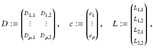
with data derivatives ![$$c_{j}:= (\partial _{t}g_{j}(x^{i}))_{i\in [n]}$$](/wp-content/uploads/2016/04/A183156_2_En_38_Chapter_IEq71.gif) and
and ![$$D_{j,k}:= \text{diag}\left ((\partial _{k}g_{j}(x^{i}))_{i\in [n]}\right )$$](/wp-content/uploads/2016/04/A183156_2_En_38_Chapter_IEq72.gif) . The matrix operator L l, k applied to variable u approximates the spatial derivative ∂ k of the flow component u l using the 2-tap linear filter { − 1, +1} and Neumann boundary conditions.
. The matrix operator L l, k applied to variable u approximates the spatial derivative ∂ k of the flow component u l using the 2-tap linear filter { − 1, +1} and Neumann boundary conditions.

(64)

(65)
![$$c_{j}:= (\partial _{t}g_{j}(x^{i}))_{i\in [n]}$$](/wp-content/uploads/2016/04/A183156_2_En_38_Chapter_IEq71.gif) and
and ![$$D_{j,k}:= \text{diag}\left ((\partial _{k}g_{j}(x^{i}))_{i\in [n]}\right )$$](/wp-content/uploads/2016/04/A183156_2_En_38_Chapter_IEq72.gif) . The matrix operator L l, k applied to variable u approximates the spatial derivative ∂ k of the flow component u l using the 2-tap linear filter { − 1, +1} and Neumann boundary conditions.
. The matrix operator L l, k applied to variable u approximates the spatial derivative ∂ k of the flow component u l using the 2-tap linear filter { − 1, +1} and Neumann boundary conditions.Solving
Objective function (64) is strictly convex in u under mild conditions [33], and thus a global minimum of this problem can be determined by finding a solution to ∇ u E(u) = 0. This condition explicitly reads

which is a linear equation system of size 2n in  with a positive definite and sparse matrix. A number of well-understood iterative methods exist to efficiently solve this class of problems even for large n [45].

(66)
 with a positive definite and sparse matrix. A number of well-understood iterative methods exist to efficiently solve this class of problems even for large n [45].
Examples
Figure 9 illustrates the method by Horn and Schunck for a small synthetic example. The choice of parameter σ is a trade-off between smoothing out motion boundaries (see Fig. 9b) in the true flow field (Fig. 9a) and sensitivity to noise (Fig. 9d).


Fig. 9
(a) Synthetic flow field used to deform an image. (b)–(d) Flow field estimated by the approach by Horn and Schunck with decreasing strength of the smoothness prior
Probabilistic Interpretation
Considering E(u) as a the log-likelihood function of a probability density function gives rise to the maximum a posteriori interpretation of the optimization problem (56), i.e.,

As E(u) is quadratic and positive definite due to the assumptions made in section “Solving,” this posterior is a Gaussian multivariate distribution

with precision (inverse covariance) matrix  and mean vector
  that solves (66).

(67)

(68)
 and mean vector
  that solves (66).
Examining the conditional distribution of  allows to quantify the sensitivity of u. To this end a permutation matrix
  , Q ⊤ Q = I, is defined such that u i = Q i u. Then, fixing
  leads to

with  and
and

Using the matrix inversion theorem to invert Σ block wise according to Q and restricting the result to u i reveals

Comparison of (70) to (71) and further analysis yield (for non-boundary pixels)

with S i = S(x i ) as defined by (59). Consequently, smaller values of σ reduce the sensitivity of u i , but some choice σ > 0 is inevitable for singular S i .
 allows to quantify the sensitivity of u. To this end a permutation matrix
  , Q ⊤ Q = I, is defined such that u i = Q i u. Then, fixing
  leads to
(69)
 and
and
(70)

(71)

(72)
Data Terms
Handling Violation of the Constancy Assumption
The data term as proposed by Horn and Schunck was refined and extended in literature in several ways with the aim to cope with the challenging properties of image data of real applications; see section “Basic Difficulties of Motion Estimation.”
Changes of the camera viewpoint as well as moving or transforming objects may cause previously visible image features to disappear due to occlusion, or vice versa to emerge (disocclusion), leading to discontinuous changes of the observed image features g(x(t), t) over time and thus to a violation of the invariance constraint (57).
Surface reflection properties like specular reflections that vary as the viewpoint changes, and varying emission or illumination (including shadows), also cause appearance to change, in particular in natural and outdoor scenes.
With some exceptions, most approaches do not explicitly model these cases and instead replace the quadratic distance function ρ 2 2 by the convex ℓ 2-distance or its differentiable approximation ρ 2, ε , to reduce the impact of outliers in regions with strong deviation from the invariance assumption. A number of non-convex alternatives have been proposed in the literature, including the truncated square distance ρ 2, λ , which further extend this concept and are often referred to as “robust” approaches.
Another common method is to replace the constancy assumption on the image brightness by one of the more complex feature mappings g(x, t) introduced in section “Invariance, Correspondence Problem,” or combinations of them. The aim is to gain more descriptive features that overcome the ambiguities described in section “Differential Constraint Equations, Aperture Problem,” e.g., by including color or image structure information from a local neighborhood. Furthermore, robustness of the data term can be increased by choosing features invariant to specific image transformations. For example, g(x) = ∇f(x) is immune to additive illumination changes.
Patch Features
Contrary to the strongly localized brightness feature g(x) = f(x), local image patches sampled from a neighborhood  of x,
of x,


 of x,
of x,
(73)
Stay updated, free articles. Join our Telegram channel

Full access? Get Clinical Tree


