Fourier Transforms in Magnetic Resonance Imaging
Objectives
At the completion of this chapter, the student should be able to do the following:
• Define mathematical transform.
• Describe the use of the Fourier transform in magnetic resonance imaging (MRI).
• Identify the following concepts: spatial domain, frequency domain, and spatial frequency domain.
• Discuss how the magnetic resonance (MR) signal is located in the patient (spatial localization).
• Define the Nyquist theorem and discuss its use in MRI.
Key Terms
Jean Baptiste Joseph Fourier (1768-1830) was a French physicist and mathematician who lived at the time of the French Revolution. Among his many accomplishments is the derivation of the mathematical transform that carries his name, the Fourier transform (FT).
The FT has always played an important role in digital image processing. Until recently, this role was buried in the depths of the derivation of the computed tomography (CT) reconstruction algorithm or in more complex image quality specifications such as the modulation transfer function (MTF). However, with the appearance of magnetic resonance imaging (MRI), the FT has been called to center stage.
FT is the mathematical mechanism for changing any of the magnetic resonance (MR) signals (free induction decay [FID], spin echo [SE], or gradient echo [GRE]) into a nuclear magnetic resonance (NMR) spectrum for chemical analysis or into a diagnostic image. Therefore an understanding of this transform is necessary, especially as it relates to MRI. Among other features, the FT provides an explanation of a type of artifact encountered in MR images (i.e., aliasing).
What is a Transform?
The FT is only one of many transforms in mathematics. For an understanding of what mathematicians mean by a transform, perhaps it is best to provide an analogy.
In nature, connections between numbers always occur. For example, the length of the side of a square affects the area of the square and vice versa. With the measurement of a few squares, a pattern of values begins to appear (Table 8-1).
TABLE 8-1
The Relationship Between the Side and Area of a Square
| Side of Square | Area of Square |
| 1 | 1 |
| 2 | 4 |
| 4 | 16 |
| 8 | 64 |
| 10 | 100 |
It is obvious that the area of the square depends on the length of the side of the square. A general relationship between these quantities can be defined: to find the area of the square, multiply the length of the side of the square by itself. The area equals the square of the length of a side. This relationship between two sets of numbers is called a function. The relationship may be written as follows:
Note that this area function includes the following important properties:


 A function establishes a relationship between numbers; a transform establishes a relationship between functions.
What is the Fourier Transform?
The FT is only one of many transforms available; however, its properties make it uniquely useful in MRI. The FT can be presented in terms of graphs of functions to see how the FT changes the shape of these graphs. For example, the square wave function is transformed into the wavy function by Fourier transformation (Figure 8-1). The symbol FT in the figure indicates this mathematical formulation.
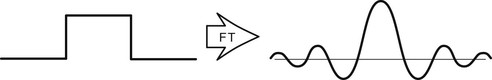
The FT has properties analogous to the area-of-a-square function discussed previously. The FT gives a unique result; for example, the square function (or boxcar function) of Figure 8-1 is Fourier transformed only into the wavy function shown. This wavy function is called a sinc function or sin x/x. The amplitude and width of the square function are related to the amplitude and wavelength of the sinc function.
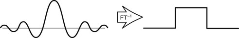
Because the FT is unique, a unique inverse FT also exists. Only one function can produce the wavy function of Figure 8-1; that is, the FT can be undone so that the original function is produced (Figure 8-2). The symbol FT−1 represents the inverse Fourier transform.
A mathematical formula can be written to define the FT. The exact form of this formula is unimportant, except that it contains sums of sines and cosines. Sines and cosines are oscillating functions whose effects are often seen in the FT. For example, the square function in Figure 8-1 is sharp edged, yet its FT has waves in it. These waves include sines and cosines.
The units of the source function and the resulting transformed function are different but related. If the source function is a plot of signal intensity versus time, then the Fourier transformed function is a plot of signal intensity versus 1/time (i.e., frequency).
 The FT of intensity versus time is intensity versus frequency.
Why a Transform?
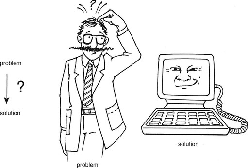
What is the use of a transform? The answer lies in the desire to solve problems. Physicists and engineers are always trying to understand the real world and how it reacts to changing situations. They write formulas to represent some part of the world, and then try to solve these formulas to see how that part will behave. For example, the response of a bridge to a crosswind can be predicted by setting up a set of equations that represent the properties of the bridge and by solving these equations in the presence of a force that represents the wind. Unfortunately, these equations are often extremely complicated, and their solution is not at all obvious (Figure 8-3).
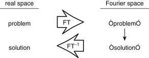
Sometimes if a transform like the FT is applied to source equations, the solution of the transformed equations is easier to obtain than the solution of the source equations. The answer to the FT of the source equation is in Fourier space. If an inverse transform is applied to the Fourier space equation, the result is in real space (Figure 8-4). This result is the same as if the problem had been solved directly. In addition, viewing the problem in Fourier space sometimes gives unique insights into the situation, insights that are not obvious in real space.
The FT does not really change the information present in a function. Rather, it represents that information in a reorganized way, offering a new viewpoint on the data. Thus the situation is viewed in either real space or Fourier space. In both spaces the same real-world thing is represented (e.g., an image, an MR signal). The FT just offers a new and unique viewpoint on these data. For example, the MR signal is a function of intensity versus time (i.e., time domain). The FT gives a representation of those same data as intensity versus frequency (i.e., the frequency domain).
The Frequency Domain
Suppose that the real-space function represents some sort of signal in time, that is, a representation of the signal intensity as it varies with time, like an MR signal. The Fourier space representation does not have the same units. The units on the horizontal axis in Fourier space are inverse of the units in real space. In this case, the horizontal real-space unit is time (e.g., seconds). Therefore the unit in Fourier space is 1/time (e.g., 1/seconds).
The quantity 1/time (e.g., cycles/second, hertz) occurs often and is frequency. A plot of intensity versus frequency is a spectrum. The FT can take a picture of intensity versus time (i.e., the time domain) and create a picture of the same signal represented as intensity versus frequency (i.e., the frequency domain).
Once again, real-space and Fourier space views are two different representations of the same real-world object. For example, the MR signal is a real-space representation of how that signal varies with time. The FT shows how the same signal varies with frequency, that is, what frequencies are present in the signal.
The concept of frequency domain or spatial frequency domain is easy to recognize. For example, ears do a frequency transformation of the signals (i.e., sounds) that they receive. The time domain representation of the sound generated by a complex source such as a symphony orchestra can be represented by a rapidly varying oscillating signal. This signal alone conveys little meaning. However, human hearing takes this time-varying signal and transforms it into frequencies.
In the complex sound from a symphony, the ear can distinguish between the high treble pitch of a violin and the deeper bass pitch of a tuba. Indeed, a small percentage of people have absolute pitch, the ability to tell the precise pitches (i.e., frequencies) of the sounds they hear. In this sense, ears “view” the world in the frequency domain.
Too Small to See
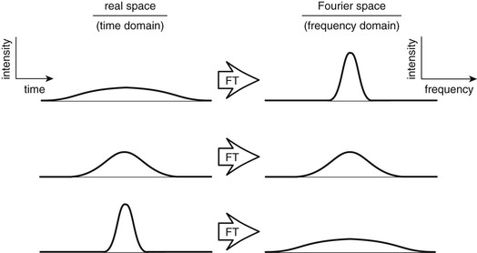
On the left side of Figure 8-5 are three smooth, bell-shaped (i.e., Gaussian) functions in real space. On the right side are their corresponding Fourier transforms. If these real-space functions represent a signal (i.e., the representation of intensity with time), then the Fourier space representation is a frequency spectrum (i.e., representation of the frequencies present).
Related posts:


Stay updated, free articles. Join our Telegram channel

Full access? Get Clinical Tree


