Fig. 11.1
Flowchart illustrating main image analyses steps involved in a typical DSS
Fig. 11.2
Flowchart illustrating the sequence of important preprocessing steps required before any MR image analyses
MRI Preprocessing: Adjusting for System Factors
MRI preprocessing is an essential first step of any sophisticated image analysis. Acquiring MR images on different platforms results in different pixel intensity ranges, image resolutions, contrast-to-noise ratios, slice thicknesses, background details, and subject orientations that makes serial and inter-subject analysis problematic. These variations may confound comparisons of image features between brain tumor types and complicate a classification task. Therefore, preprocessing of MR images is essential to ensure that any information obtained from the images is standardized, comparable, and reproducible.
Intensity Normalization Methods
Intensity normalization is the most important preprocessing step when preparing to analyze a set of MR images because many of the morphological features used in classification or serial image comparisons are directly dependent on the image intensities. Several methods have been proposed for intensity normalization of MR images with varying success. In this section, we discuss some of the most popular and widely used normalization methods.
Kullback–Leibler Divergence-Based Intensity Normalization
Wiesenfeld et al. [4] proposed a Kullback–Leibler (KL) divergence-based technique to simultaneously estimate the intensity inhomogeneity and normalize the intensities in MR images. The method assumes a multiplicative model of intensity inhomogeneity,
 where O(x, y) is the observed image, F(x, y) is the multiplicative intensity inhomogeneity, I(x, y) is the corrected image, and n(x, y) is the acquisition noise. The method assumes that the noise has very little influence on the intensity normalization. The KL divergence between the intensity inhomogeneity corrected image I ≈ F − 1 O and a target intensity histogram is iteratively minimized to estimate F(x, y),
Simultaneous perturbation stochastic approximation (SPSA) is used to generate gradient estimates of the KL-divergence. Although this method works well, pixel-wise estimation of the intensity inhomogeneity F(x, y) reduces the performance of this normalization method such that it is much slower than the other methods presented in the following sections.
Consistent Intensity Correction
Consistent intensity correction operates by matching the observed intensity histogram to a target intensity histogram [5]. The two histograms are approximated using Gaussian mixture models (GMMs) and the expectation maximization (EM) method is used to estimate the model parameters. The intensities within specific anatomical regions are aligned and interpolated using a smooth polynomial function f p (x) of order p,
The coefficients of the polynomial function θ i are estimated by minimizing the following energy function,
 where l = 1, …, n represents the anatomical regions, and μ l and v l are the mean intensity of the anatomical regions in the histogram of the image to be normalized and the target histogram, respectively. The advantage of this method is that it does not require a spatial alignment for the image(s) to be corrected. However, this method suffers from low generalizability and only average accuracy relative to other methods discussed in this section.
Intensity Normalization by Joint Histogram Registration
Jager et al. [6] proposed an intensity normalization method that minimizes a distance measure between the joint probability density functions (PDFs) of the tissue types from a set of MR images to be normalized and a set of reference images. The distance minimization is posed as a nonrigid registration problem with the images considered to be the joint PDFs. The minimization problem can be formulated as,
 where f is the deformation field mapping the PDF of the uncorrected images p U to the PDF of the reference images p R ; D(p R ,p U ;f) is a sum of squared differences (SSD) based distance measure; and S(f) is a smoothness measure. The distance measure is defined as,
 where
where  , and Ω represents the joint PDF image domain. A regularization measure based on curvature smoothness is defined as,
 with Δ(.) being the Laplacian operator, and n as the dimensionality of joint PDF. The objective function τ(p R ,p U ;f) is minimized using a variational approach. The histogram registration method is applicable for multi-modality images, but requires at least two imaging sequences (e.g., T1 and T2 weighted images). The method has been reported to perform well and is fairly generalizable [7]. However, nonrigid registration makes this method considerably slower than approaches that normalize an image without using additional preprocessing steps.
, and Ω represents the joint PDF image domain. A regularization measure based on curvature smoothness is defined as,Decile Normalization Method
Decile normalization (DN) [8, 9] is a widely used method for intensity normalization of brain MR images. This method works by setting percentile-based ten intensity landmarks (deciles) C L ,
 where each m i , i = {10,20,….,90} denotes pixel intensities of the i th percentile of the histogram corresponding to the foreground in the MR image. Since image artifacts and outliers typically have extreme image intensities, p low and, p high are used as the end percentiles instead of m 0, and m 100 to reduce sensitivity to such image corruptions. The foreground extraction is performed through a thresholding approach that uses the mean intensity of the image (for intensities between p low and p high ) as the intensity threshold. The landmarks of the template MR image C L Temp to be normalized are then transformed to landmarks calculated on a reference histogram C L Ref using a piecewise linear mapping. Piece-wise linear mapping (Fig. 11.3) helps reduce the sensitivity of normalization method to the presence of anatomical abnormalities such as lesions and treatment scars.
Fig. 11.3
Figure illustrating piecewise linear mapping between input image histogram and reference histogram
This method is very fast, easy to implement, and applicable to images from multiple modalities [8–10]. Gasser et al. [10] evaluated the effectiveness of DN on MR images containing pathology, obtained from multiple acquisition sites, scanners, and MR modalities. They quantitatively evaluated the effect of DN on tissue separation, and reported significantly improved accuracy when intensity normalization is performed.
Spatial Normalization
The spatial location of brain tissue often does not correlate well across images and varies among different MR acquisitions. The variations in spatial location of brain tissue are due to differences in acquisition parameters, patient placement in the scanner, and patient motion. Therefore, spatial normalization is an important preprocessing step required before any comparison studies can be done. These can be both interpatient comparisons (between different patients) and intra-patient comparisons (change detection during follow-up to evaluate treatment outcomes). The spatial normalization involves alignment of MR imaging data to a standard reference dataset of images using image registration. The reference set of images used in existing normalization methods is often chosen as corresponding to tissue probability maps (Fig. 11.4). The alignment of imaging data to tissue probability maps has the additional benefit in brain tissue segmentation of introducing tissue-specific priors into probability-based models often used for voxel classification.
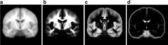
Fig. 11.4
Figure showing (a) template image, and probabilistic atlas maps of (b) white matter, (c) gray matter, and (d) cerebrospinal fluid obtained from International Consortium for Brain Mapping (ICBM)
Spatial normalization using image registration is a difficult task since MR images may have been captured through multiple modalities and is further complicated by the presence of anatomical deviations in the brain such as pathology, resection scars, and treatment side effects. In this section, we discuss some of the most commonly used spatial normalization methods for brain MR images.
Unified Segmentation
Image registration is affected by changes in image intensities due to corruptions such as noise, intensity inhomogeneity, and partial volume effects. Unified segmentation combines the three interdependent tasks of segmentation, intensity inhomogeneity correction, and spatial normalization under the same iterative formulation [11]. As a rough fit, a tissue probability map is first aligned to the patient data using affine registration. The initial alignment is further refined using nonlinear deformations, which are modeled as linear combinations of discrete cosine transform basis functions. This spatial normalization is combined with the task of image segmentation using a principled Bayesian probabilistic formulation that utilizes tissue probability maps as priors. The intensity inhomogeneity correction is included within the segmentation model to account for smoothly varying intensities across the image domain. Once the method converges, the inverse of the transformation that aligns the tissue probability maps to the patient data can be used to normalize the patient MR images.
Diffeomorphic Anatomical Registration Through Exponentiated Lie Algebra
Diffeomorphic anatomical registration through exponentiated lie algebra (DARTEL) is another such normalization method that depends on image segmentation [12]. The reference imaging data is deformed to align them to the patient MR imaging data. However, unlike unified segmentation, DARTEL includes a much higher number of parameters in registration, which enables the modeling of more detailed and finer deformations. In DARTEL, the deformations are modeled using a flow field that is assumed to be constant in time. This enables a one-to-one inverse mapping of the deformation field from the reference imaging data that can be used for normalization of patient MR imaging data. DARTEL has been reported to be superior to unified segmentation for spatial normalization of MR images, including those with anatomical deviations such as tumors and resection scars [13, 14].
Automatic Registration Toolbox
Automatic registration toolbox (ART) [15] is based on a multi-scale neighborhood search to find the most similar image voxel between the patient MR images {I P (v), v ∈ Ωp} and the reference images {I R (v), v ∈ ΩR}, where v corresponds to the image voxels belonging to image domains Ωp and ΩR, respectively. The patient MR images are resized and interpolated to match the dimensions of the reference MR data, followed by a neighborhood-based voxel search in the reference image. A similarity metric S(w 1, w 1) between two vectors w 1 and w 1 is defined as,
 where H is an idempotent symmetric centering matrix that removes the mean of the vector it pre-multiplies. For every voxel v i in patient MR data, vector w 1 is defined as a vector of voxel intensities that are in a neighborhood
  around
  . The corresponding voxel in the reference MR data I R can be found by searching in a finite neighborhood ψ i around and including voxel location v i . Let voxel v j ∈ ψ i be the voxel in this neighborhood when the similarity measure
  is maximum,
around . The corresponding voxel in the reference MR data I R can be found by searching in a finite neighborhood ψ i around and including voxel location v i . Let voxel v j ∈ ψ i be the voxel in this neighborhood when the similarity measure is maximum,The initial estimate of the displacement field for voxel v i is w(i) = j − i. The estimation is further refined by computing the displacement field at multiple resolution levels using the scale-space theory. In comparison studies performed on normal subjects, ART has been reported superior to other methods for reducing inter-subject anatomical variability [13, 15].
MRI Preprocessing: Adjusting for Patient Factors
The presence of noise and other image artifacts is often prominent in MRI and adversely affects any attempts at quantitative image analysis. The correction of such image corruptions is also an essential part of the image preprocessing required before any quantitative feature extraction can be performed. In this chapter, we divide preprocessing steps into two categories based on the source of the problem. While the methods discussed in section “MRI Preprocessing: Adjusting for System Factors” dealt specifically with problems that arise solely from system factors, this section deals with image corruptions that result from the combined effect of system and patient factors.
This raises the question of the sequence in which these two categories of preprocessing methods should be carried out. Both image normalization and removal of image corruptions utilize image intensity information and therefore are interdependent tasks. Madabhushi and Udupa [16] in an analysis of nearly 4,000 cases suggested that noise and artifact removal should precede image normalization. They also demonstrated that iterative adjustment of system and patient factors, as is often done, does not considerably improve the image quality (Fig. 11.2).
Image De-Noising
As with other medical imaging modalities, MR images contain significant amounts of noise that compromise the performance of the image analyses incorporated into any DSS. The main causes of noise in MRI are due to thermally driven Brownian motion of electrons within patient’s conducting tissue (patient factor) and within reception coil (system factor). There is a trade-off between spatial resolution, signal-to-noise ratio (SNR), and acquisition time in MRI. While SNR can, in principle, be improved by increasing the acquisition time it is not a practical solution to implement in the clinic. Therefore, there is a need for de-noising algorithms that can improve image quality and reduce image noise after image acquisition.
Several de-noising algorithms have been proposed in the literature that are based on methods adapted from either general image processing or developed specifically for MRI specific noise. The distribution of noise in MR images is known to follow a Rician distribution, which, unlike Gaussian noise, is signal dependent and therefore much harder to remove. The noise in MR images is introduced during the calculation of the magnitude image from the complex Fourier domain data collected during an MRI scan. In this section, we discuss some of the most widely used de-noising methods in MRI.
Anisotropic Diffusion
Anisotropic diffusion is a widely used adaptive de-noising method that only locally smoothes the continuous regions of an image, while preserving the edges/boundaries between the image regions. The anisotropic diffusion model is defined by,
 where u(x,y,t) represents an image parameterized with the spatial coordinates (x, y) and an artificial time t that represents the number of smoothing iterations; div(.), Δ(.) and ∇(.) are the divergence, the Laplacian, and the gradient operators, respectively; g(∣∇u(x,y,t)∣2) is a diffusivity term that controls the strength of smoothing. The following diffusivities g(∣∇u(x,y,t)∣2) were proposed by Perona and Malik [17],
 where λ < 0 is a scaling parameter that controls the edge enhancement threshold. Anisotropic diffusion works well for natural images with well-defined boundaries; however, their use in MR images is limited due to the presence of partial volume effects that result in smooth region boundaries.
Wavelet Analysis
In wavelet analysis, an image u(x,y) is decomposed into discrete wavelets at different scales and translations defined as,
 where Ψ j,k (x,y) are the wavelet basis functions, and j and k are the scale and translation parameters, respectively, and d j,k are the wavelet mixing coefficients estimated by,
De-noising an image with wavelet analysis involves thresholding wavelet coefficients d j,k to discard coefficients that do not have significant energy. Although successful in removing noise, wavelet-based methods do not preserve the finer details in MR images and thus further exacerbating any partial volume effects.
Rician-Adapted Non-Local Means Filter
The non-local (NL) means filter [18] removes noise by computing a weighted average of surrounding pixels. The weights are determined using a similarity measure between local neighborhoods around the pixels being compared. The NL-corrected version of an image u(x) can be represented as,
 where S i represents the size of the neighborhood around any pixel x i to be used to compute the weighted average. w(x i , x j ) are the assigned weights to pixels x j belonging to space S i defined as,
![$$ w\left({x}_i,{x}_j\right)=\frac{1}{Z_i} exp\left(-\frac{\left|\right|u\left({N}_i\right)-u\left({N}_j\right)\left|\right|{}^2}{h^2}\right),\kern1em w\left({x}_i,{x}_j\right)\in \left[0,1\right] $$](/wp-content/uploads/2016/03/A218098_1_En_11_Chapter_Equp.gif) where Z i is a normalization constant such that
where Z i is a normalization constant such that  , h is a decay parameter determining the rate of decay in weighting, and N i is the neighborhood image patch centered around pixel x i of radius r.
, h is a decay parameter determining the rate of decay in weighting, and N i is the neighborhood image patch centered around pixel x i of radius r.Wiest-Daessle [19] proposed a Rician-adapted version of this NL-means filter using the properties of the second-order moment of a Rice law,
 where σ is the variance of the Gaussian noise in the complex Fourier domain of MR data and is estimated using pseudo-residual technique proposed by Gasser et al. [10].
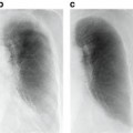
Rician-adapted NL-means filter has been reported to outperform wavelet analysis, Gaussian smoothing, and anisotropic diffusion for de-noising MR images with Rician noise distribution [20–22] (Fig. 11.5).
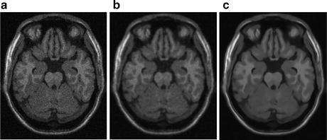
Fig. 11.5
Figure showing (a) sample MR image with Rician noise, (b) denoised image with anisotropic diffusion, and (c) denoised image obtained from Rician-adapted NLM filter
Removal of MRI Artifacts
MR images suffer from several image artifacts such as partial volume effects, Gibbs’s artifacts, chemical shifting, motion artifacts, and intensity inhomogeneities. These artifacts often produce an abnormal distribution of intensities in the image, thereby compromising the accuracy of automatic image analysis methods. Though some artifacts can be corrected during the image reconstruction phase, other artifacts must be corrected through post-acquisition image processing. In this section, we will discuss some of the post-processing methods to deal with partial volume effects and intensity inhomogeneities, two of the most prominent and widely studied artifacts that require post-processing.
Intensity inhomogeneity, also known as intensity nonuniformity (INU), the bias field, or shading, is one of the most prominently occurring artifacts in MR images. This adverse phenomenon appears as smooth intensity variations across the image domain (Fig. 11.6), which results in the intensity of voxels belonging to the same class varying with location within the image. INU artifacts in MR images are mostly due to acquisition imperfections such as nonuniform RF excitation, nonuniform coil receptor sensitivity, and standing wave effects [23]. Other minor factors that may also produce INU effects include eddy currents due to rapid switching of magnetic field gradients; patient-induced electromagnetic interactions, and geometric distortions. The INU artifacts become much more significant when scanners are operating at higher strength magnetic field strengths. Although INU artifacts have little effect on visual interpretation of an MR image by a radiologist, they significantly degrade the performance of automatic image analysis methods. For this reason, INU correction has been an active field of research and a number of methods have been proposed in the literature.
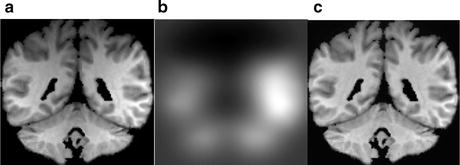
Fig. 11.6
Figure showing real MR image (a) corrupted from intensity inhomogeneity, (b) estimated intensity inhomogeneity, and (c) recovered image
The correction of intensity inhomogeneities can be broadly classified into: prospective and retrospective methods. Prospective correction requires special imaging sequences with physical phantoms and multiple reception coils and involves recalibrating the scanner based on an assessment of the excitation field strength and the nonuniformity in reception coils. Although prospective methods can potentially correct for static INU artifacts resulting from scanner imperfections, they are unable to account for patient-induced intensity inhomogeneities. Furthermore, the longer scanning routines typically involved in prospective correction methods make them impractical in clinical settings. Retrospective correction, on the other hand, uses the intensity information contained within an acquired image to estimate INU artifacts and is therefore a more general solution than prospective correction. This makes them much more useful for clinical use; however, they are unable to distinguish between scanner and patient-induced intensity inhomogeneities.
Spectrum Filtering Methods
Due to their slowly varying nature across image domain, correction methods generally assume that INU artifacts are low-frequency signals that can be removed from the higher frequency spectrum of anatomical structures. The two main filtering approaches are homomorphic filtering and homomorphic unsharp masking.
Homomorphic filtering takes the difference between the log transformed image log(I(x,y)) and a low-pass filtered (LPF) version of the logarithmic image, with a mean-preserving normalization constant (C) [24]. The corrected image  can be obtained by taking the exponential of the difference image,

can be obtained by taking the exponential of the difference image,Homomorphic unsharp masking corrects an image by dividing the acquired image I(x, y) with the LPF version of the image, scaled by a mean-preserving normalization constant [25].
Although widely used, low-pass filtering methods are thought to have rather limited ability to correct for INU artifacts in brain MR images. The limited effectiveness of these methods is due to the significant overlap of the frequency spectrums of INU artifacts and brain structures, which does not fit the assumption underlying these techniques.
Intensity Histogram-Based Methods
Histogram-based methods operate on the principle that the information content in an image is changed by artifacts such as intensity inhomogeneities. Sled et al. [26] proposed a non-parametric nonuniformity normalization (N3) method that iteratively corrects for INU artifacts by maximizing the frequency content of the intensity distributions in the corrected image. N3 is a fully automated method, does not include any assumptions about the anatomical structures present, and has been reported to be one of the most successful methods for INU correction.
Histogram-based methods have also been developed that propose the information content of an image increases when corrupted by INU artifacts. These methods assume that INU artifacts can be corrected by minimizing the entropy (information content) of the image, subject to some constraints. Several researchers have explored this concept by minimizing energy functions that combine image entropy, INU smoothness constraints and mean-preserving regularization terms to correct for INU artifacts [27–30]. An advantage is that these information minimization methods are highly generalizable and thus can be used on any MR image.
Spline Fitting Methods
The smooth varying nature of INU artifacts has motivated the use of polynomial and spline surfaces on a set of extracted image features to estimate INU artifacts. In these methods, a spline function is least squares fitted to a set of image pixels belonging to a major tissue type and distributed throughout the image. Both manual and automatic candidate image feature selection methods have been investigated, and manual selection was reported to be more accurate than automatic selection [31]. A major limitation of this approach is the extrapolation of INU computed from a single tissue class to estimate the INU artifacts across the entire image. This framework may be sufficient to correct INU artifacts due to scanner imperfections, but patient-induced INU artifacts that may vary between tissue types are not handled appropriately. The time-consuming manual selection of points in every image slice is another limitation, and also potentially introduces user subjectivity.
INU Correction Combined with Brain Tissue Segmentation
Combining INU correction with image segmentation is commonly used for retrospective correction of intensity inhomogeneities in MR images. INU correction and image segmentation depend on one another, and, therefore, better segmentation and INU correction can be achieved by simultaneously utilizing information from these tasks. Furthermore, one result of these approaches is brain tissue segmentation, which is often essential for subsequent quantitative MR image analysis. A common theme of these methods is the minimization/maximization of an objective function that contains a data fitting term that is regularized with an INU artifact smoothness term.
Several probabilistic approaches using maximum likelihood (ML) and maximum a posteriori (MAP) have been proposed to define data fitting terms for image voxel classification. The intensity distributions inside each image region are modeled using assumed parametric models that incorporate effects from intensity corruptions due to INU. A common choice of parametric models has been the finite Gaussian mixture (FMM) models over the image domain with the model parameters estimated using popular expectation maximization (EM) algorithm. FMM are often defined with every tissue class described using a single Gaussian component [32, 33], or as a combination of multiple components [34–36]. The class priors are often included to improve the segmentation and INU artifact estimation using either probabilistic atlases or hidden Markov random field (HMRF) defined priors. Other approaches have also been proposed including non-parametric segmentation based on max–shift and mean–shift clustering for INU estimation [37, 38], and fuzzy C-means (FCM)-based methods that assume each voxel can belong to multiple tissue classes. Since there is significant overlap in the algorithms used for segmentation and INU estimation, we refer readers to see “Brain Tissue Segmentation” section of this chapter.
The data fitting term is regularized with a smoothness term that ensures that the estimate INU artifact is smoothly varying across the image domain. The smoothness term is often defined in terms of the first and second order derivatives of the intensity inhomogeneity field. The minimization of the smoothness term accounts for the smoothly varying nature of INU artifacts in MR images. For numerical convenience, polynomial and spline surfaces have been widely used for modeling intensity inhomogeneity. When combined with the tissue segmentation process, selection of candidate points can be performed automatically. This addresses the major limitation suffered by spline fitting methods as discussed in earlier sections.
Brain Tissue Segmentation
Segmentation of brain MR images into tissue types is often an important and essential task in the study of many brain tumors. It enables quantification of neuroanatomical changes in different brain tissues, which may be informative for diagnosis and treatment follow-up of brain tumor patients. Besides brain tumors, brain tissue segmentation is useful in management of neurodegenerative and psychiatric disorders such as schizophrenia, and epilepsy. Multiple sclerosis (MS), for instance, requires accurate quantification of lesions in the white matter part of the brain for assessment of drug treatment. Even though MRI produces high quality volumetric images, the presence of image corruptions (noise, intensity inhomogeneities, and partial-volume effects) makes the segmentation of brain MR images complicated and challenging. Due to these reasons, brain MR segmentation has been an active field of research with a variety of methods proposed in literature. Traditional methods such as image thresholding and region growing usually fail due to the complex distribution of intensities in medical images. Furthermore, the presence of intensity inhomogeneity and noise significantly impact these intensity-based methods. In this section, we discuss some of the most widely explored methods for medical image segmentation.
Fuzzy C-Means-Based Segmentation Methods
FCM is based on calculating fuzzy membership of image voxels to each of multiple classes. The following objective function is iteratively minimized,
 where w i,j k is the fuzzy membership of observation x i in cluster c j satisfying ∑ C j = 1 w
 Computational Intelligent Image Analysis for Assisting Radiation Oncologists’ Decision Making in Radiation Treatment Planning
 The Role of Content-Based Image Retrieval in Mammography CAD
 Liver Volumetry in MRI by Using Fast Marching Algorithm Coupled with 3D Geodesic Active Contour Segmentation
 Computational Anatomy in the Abdomen: Automated Multi-Organ and Tumor Analysis from Computed Tomography
 Subtraction Techniques for CT and DSA and Automated Detection of Lung Nodules in 3D CT
 Bone Suppression in Chest Radiographs by Means of Anatomically Specific Multiple Massive-Training ANNs Combined with Total Variation Minimization Smoothing and Consistency Processing


Related posts:
Computational Intelligent Image Analysis for Assisting Radiation Oncologists’ Decision Making in Radiation Treatment Planning
The Role of Content-Based Image Retrieval in Mammography CAD
Liver Volumetry in MRI by Using Fast Marching Algorithm Coupled with 3D Geodesic Active Contour Segmentation
Computational Anatomy in the Abdomen: Automated Multi-Organ and Tumor Analysis from Computed Tomography
Subtraction Techniques for CT and DSA and Automated Detection of Lung Nodules in 3D CT
Bone Suppression in Chest Radiographs by Means of Anatomically Specific Multiple Massive-Training ANNs Combined with Total Variation Minimization Smoothing and Consistency Processing
Stay updated, free articles. Join our Telegram channel
Full access? Get Clinical Tree
