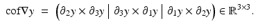
Fig. 1
Transforming a square into a disc: template image  is a white square on black background (left), reference image
  is a white disk on black background (not displayed), the transformation y is visualized by showing a regular grid X as overlay on the deformed image
 ![$$\mathcal{T} [y]$$](/wp-content/uploads/2016/04/A183156_2_En_39_Chapter_IEq3.gif) (right) and as y(X) on the template image (center); note that
(right) and as y(X) on the template image (center); note that  = \mathcal{T} (y(x))$$](/wp-content/uploads/2016/04/A183156_2_En_39_Chapter_IEq4.gif)
is a white square on black background (left), reference image is a white disk on black background (not displayed), the transformation y is visualized by showing a regular grid X as overlay on the deformed image (right) and as y(X) on the template image (center); note that This chapter presents a comprehensive overview of mathematical techniques used for nonlinear image registration. A particular focus is on regularization techniques that ensure a mathematically sound formulation of the problem and allow stable and fast numerical solution.
Starting out from one of the most commonly used linear elastic models [10, 55], its limitations and extensions to nonlinear regularization functionals based on the theory of hyperelastic materials are discussed. A detailed overview of the available theoretical results is given and state-of-the-art numerical schemes as well as results for real-life medical imaging applications are presented.
2 The Mathematical Setting
The purpose of this section is to provide a brief, conceptual introduction to a variational formulation of image registration, see section “Variational Formulation of Image Registration”. For brevity, the presentation is restricted to a small subset of the various configurations of the variational problem and is limited to 3D problems which today is most relevant in medical imaging applications. Section “Images and Transformation” defines a continuous model for images and formalizes the concept of transformations y and transformed images ![$$\mathcal{T} [y]$$](/wp-content/uploads/2016/04/A183156_2_En_39_Chapter_IEq5.gif) . Section “Length, Area, and Volume Under Transformation” discusses the transformation of length, area, and volume. These geometrical quantities play an important role for the computation of locally invertible transformations, which are important for many clinical applications.
. Section “Length, Area, and Volume Under Transformation” discusses the transformation of length, area, and volume. These geometrical quantities play an important role for the computation of locally invertible transformations, which are important for many clinical applications.
. Section “Length, Area, and Volume Under Transformation” discusses the transformation of length, area, and volume. These geometrical quantities play an important role for the computation of locally invertible transformations, which are important for many clinical applications.After having discussed the general concepts on a rather broad level, specific building blocks of the variational framework are examined in more detail. Section “Distance Functionals” introduces two common choices of distance functionals  , which measures the alignment of the images. After motivating the demand for regularization by illustrating the ill-posedness of the variational problem in section “Ill-Posedness and Regularization”, an overview of elastic regularization functionals and a discussion of their limitations is given in section “Elastic Regularization Functionals”.
, which measures the alignment of the images. After motivating the demand for regularization by illustrating the ill-posedness of the variational problem in section “Ill-Posedness and Regularization”, an overview of elastic regularization functionals and a discussion of their limitations is given in section “Elastic Regularization Functionals”.Motivated by the limitations of elastic regularization functionals extensions to hyperelastic functionals, designed to ensure invertible and reversible transformations, are presented in section “Hyperelastic Regularization Functionals”. Subsequently, section “Constraints” presents two examples that demonstrate how constraints  can be used to restrict set of admissible transformations
  , to favor practically relevant solutions, and most importantly, to exclude practically infeasible solutions.
can be used to restrict set of admissible transformations , to favor practically relevant solutions, and most importantly, to exclude practically infeasible solutions.Finally, a comprehensive overview of related literature and suggestions for further readings are provided in section “Related Literature and Further Reading”.
Variational Formulation of Image Registration
Given the so-called template image  and the so-called reference image
  , the image registration problem can be phrased as a variational problem. Following [55], an energy functional
  is defined as a sum of the data fit
  depending on the input images and the transformation and a regularization
  ,
,
![$$\displaystyle{ \mathcal{J} [y]:= \mathcal{D}[\mathcal{T},\mathcal{R};y] + \mathcal{S}[y]. }$$](/wp-content/uploads/2016/04/A183156_2_En_39_Chapter_Equ1.gif)
The objective is then to find a minimizer y of  in a feasible set
  to be described,
![$$\displaystyle{ \min \mathcal{J} [y]\quad \mbox{ for}\quad y \in \mathcal{A}. }$$](/wp-content/uploads/2016/04/A183156_2_En_39_Chapter_Equ2.gif)
Advantages of this formulation are its great modelling potential and its modular setting that allows to obtain realistic models tailored to essentially any particular application.
and the so-called reference image , the image registration problem can be phrased as a variational problem. Following [55], an energy functional is defined as a sum of the data fit depending on the input images and the transformation and a regularization ,(1)
in a feasible set to be described,(2)
Images and Transformation
This section introduces a continuous image model, transformations, and discusses geometrical transformations of images. Although the image dimension is conceptually arbitrary, the description is restricted to 3D images for ease of presentation.
Definition 1 (Image).
Let  be a domain, i.e., bounded, connected, and open. An image is a one-time continuously differentiable function
  compactly supported in Ω. The set of all images is denoted by
  .
.
be a domain, i.e., bounded, connected, and open. An image is a one-time continuously differentiable function compactly supported in Ω. The set of all images is denoted by .Note that already a simple transformation of an image such as a rotation requires a continuous image model. Therefore, a continuous model presents no limitation, even if only discrete data is given in almost all applications. Interpolation techniques are used to lift the discrete data to the continuous space; see, e.g., [55] for an overview. As registration is tackled as an optimization problem, continuously differentiable models can provide numerical advantages.
Definition 2 (Transformation).
Let  be a domain. A transformation is a function
  . For a differentiable transformations, the Jacobian matrix is denoted by
 The function
  satisfying y(x) = x + u(x) is called displacement,
  , where I denotes a diagonal matrix of appropriate size with all ones on its diagonal.
be a domain. A transformation is a function . For a differentiable transformations, the Jacobian matrix is denoted by satisfying y(x) = x + u(x) is called displacement, , where I denotes a diagonal matrix of appropriate size with all ones on its diagonal.Example 1.
An important class of transformations are rigid transformations. Let  describes a translation and
  a rotation matrix,
 A transformation y is rigid on Σ, if
  .
.
describes a translation and a rotation matrix,.Given an image  and an invertible transformation y, there are basically the Eulerian or Lagrangian way to define the transformed version
 ![$$\mathcal{T} [y]$$](/wp-content/uploads/2016/04/A183156_2_En_39_Chapter_IEq27.gif) ; see [38, 55] for more details. In the Eulerian approach the transformed image is defined by
; see [38, 55] for more details. In the Eulerian approach the transformed image is defined by
![$$\displaystyle{ \mathcal{T} [y]: \mathbb{R}^{3} \rightarrow \mathbb{R},\quad \mathcal{T} [y](x):= \mathcal{T} (y(x)). }$$](/wp-content/uploads/2016/04/A183156_2_En_39_Chapter_Equ4.gif)
In other words, assigning position x in ![$$\mathcal{T} [y]$$](/wp-content/uploads/2016/04/A183156_2_En_39_Chapter_IEq28.gif) the intensity of
the intensity of  at position y(x); see illustration in Fig. 1. The Lagrangian approach transports the information
  to
to  , where the first entry denotes location and the second intensity. In image registration, typically, the Eulerian framework is used. However, the Lagrangian framework can provide advantages in a constrained setting; see [38] for a local rigidity constrained and the discussion in section “Constraints”.
and an invertible transformation y, there are basically the Eulerian or Lagrangian way to define the transformed version ; see [38, 55] for more details. In the Eulerian approach the transformed image is defined by(3)
the intensity of at position y(x); see illustration in Fig. 1. The Lagrangian approach transports the information to , where the first entry denotes location and the second intensity. In image registration, typically, the Eulerian framework is used. However, the Lagrangian framework can provide advantages in a constrained setting; see [38] for a local rigidity constrained and the discussion in section “Constraints”.Length, Area, and Volume Under Transformation
This section relates changes of length, area, and volume in the deformed coordinate system to the gradient of the transformation y. To simplify the presentation, it is assumed that y is invertible and at least twice continuously differentiable.
Using Taylor’s formula [18], a local approximation of the transformation at an arbitrary point x in direction  is given by
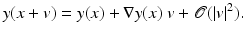
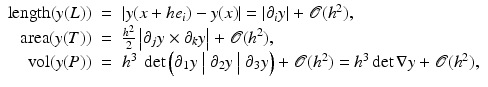
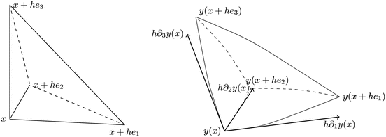
Choosing v = he i , it can be seen that the columns of the gradient matrix ∇y(x) approximate the edges of the transformed reference element; see also Fig. 2. Thus, changes of length, area, and volume of a line segment L connecting x and x + he i , a triangle T spanned by x, x + he j , and x + he k , and a tetrahedron P spanned by x and the three scaled Euclidean vectors are approximately
 where × denotes the outer product in
  .
.
is given by(4)
.Fig. 2
Visualization of a deformation of a tetrahedron and the Taylor approximation of the transformation y. At an arbitrary point x a tetrahedron is spanned by the scaled Euclidean unit vectors (left). The edges of the deformed tetrahedron are approximated by the columns of the gradient ∇y(x) (right). Due to this approximation property, geometric quantities such as volume, area, and length can be related to the gradient matrix, its cofactor, and its determinant
The cofactor matrix cof∇y summarizes, column wise, the area changes of the three triangles spanned by x with two scaled Euclidean vectors each,
 At this point, the importance of limiting the range of det∇y for many clinical applications should be stressed. Due to the inverse function theorem [25, Sect. 5], a transformation
 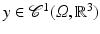 is locally one-to-one if det∇y ≠ 0. From the above considerations, it can be seen that det∇y = 0 indicates annihilation of volume and det∇y < 0 indicates a change of orientation. Thus, controlling the range of det∇y, or analogously the range of compression and expansion of volume, ensures local invertibility and thus is of utmost importance in practical applications.
is locally one-to-one if det∇y ≠ 0. From the above considerations, it can be seen that det∇y = 0 indicates annihilation of volume and det∇y < 0 indicates a change of orientation. Thus, controlling the range of det∇y, or analogously the range of compression and expansion of volume, ensures local invertibility and thus is of utmost importance in practical applications. Distance Functionals
The variational formulation of the image registration problem (2) characterizes an optimal transformation as a minimizer of the sum of a distance and a regularization functional subject to optional constraints. These three building blocks will be introduced and discussed in the following sections.
Distance functionals mimic the observer’s perception to quantify the similarity of images. In the following, two examples of distance measures will be presented and the reader is referred to [55] for further options. Emphasis is on a mass-preserving distance measure, which is an attractive option for the registration of density images such as Positron Emission Tomography (PET) images; see also section “Motion Correction of Cardiac PET”.
A robust and widely use distance measure is the L 2-norm of the intensity differences commonly referred to as the sum-of-squared-difference (SSD),
![$$\displaystyle{ \mathcal{D}^{{\mathrm{SSD}}}[y] = \mathcal{D}^{{\mathrm{SSD}}}[\mathcal{T},\mathcal{R};y] = \frac{1} {2}\int _{\varOmega }(\mathcal{T} (y(x)) -\mathcal{R}(x))^{2}dx. }$$](/wp-content/uploads/2016/04/A183156_2_En_39_Chapter_Equ8.gif)
For this distance measure to be effective, intensity values at corresponding points in the reference and template image are assumed to be equal. This assumption is often satisfied when comparing images of the same modality, commonly referred to as mono-modal registration. Hence,  is a prototype of mono-modal distance functionals.
(5)
is a prototype of mono-modal distance functionals.In some applications intensities at corresponding points differ conceptually. Typical examples of multimodal image registration include the fusion of different modalities like anatomy (such as CT or MRI) and functionality (such as SPECT or PET); see, e.g., [55] for further options and discussions.
Mass densities are another example for conceptional different image intensities. The necessity of mass-preserving transformations was first discussed in [29]. Recently, mass-preserving distance functionals were used to register images from Positron Emission Tomography (PET); see section “Motion Correction of Cardiac PET” and [14, 30, 60]. Another application is the correction of image distortions arising from field inhomogeneities in Echo-Planar Magnetic Resonance Imaging; see section “Susceptibility Artefact Correction of Echo-Planar MRI” and [15, 62].
Due to mass-preservation, change of volume causes change of intensities. Note that the simple model for transformed images (3) does not alter image intensities. Let V ⊂ Ω denotes a small reference volume. Ideally, the mass of  contained in V has to be equal to the mass of
  contained in y(V ). Formally,
where the second equality holds by the transformation theorem [18, p. 31f], assuming that the transformation is injective, continuously differentiable, orientation preserving, and that its inverse is continuous. A natural mass-preserving extension of the SSD distance functional thus reads
![$$\displaystyle{ \mathcal{D}^{{\mathrm{MP}}}[y]:= \frac{1} {2}\int _{\varOmega }(\mathcal{T} (y(x)) \cdot \det \nabla y(x) -\mathcal{R}(x))^{2}\ dx. }$$](/wp-content/uploads/2016/04/A183156_2_En_39_Chapter_Equ10.gif)
contained in V has to be equal to the mass of contained in y(V ). Formally,(6)
(7)
Ill-Posedness and Regularization
A naive approach to image registration is to simply minimize the distance functional  with respect to y. However, this is an ill-posed problem [23, 27, 46, 55]. According to Hadamard [41], a problem is well-posed, if there exists a solution, the solution is unique, and the solution depends continuously on the data. If one of these criteria is not fulfilled, the problem is called ill-posed.
with respect to y. However, this is an ill-posed problem [23, 27, 46, 55]. According to Hadamard [41], a problem is well-posed, if there exists a solution, the solution is unique, and the solution depends continuously on the data. If one of these criteria is not fulfilled, the problem is called ill-posed.In general, existence of a minimizer of the distance functional cannot be expected. Even the rather simple SSD distance functional (5) depends in a non-convex way on the transformation; for a discussion of more general distance functionals, see [55, p. 112]. If the space of plausible transformations is infinite dimensional, existence of solutions is thus critical.
A commonly used approach to bypass these difficulties and to ensure existence is to add a regularization functional that depends convexly on derivatives of the transformation [10, 67, 68]. This strategy is effective for distance functionals are independent of or depend convexly on the gradient of the transformation. This is the case in most applications of image registration, for instance, for the SSD in (5). However, further arguments are required for the mass-preserving distance functional in (7) due to the non-convex of the determinant; see Sect. 1.
It is also important to note that distance functionals may be affected considerably by noise; see also [55]. This problem is often (partially) alleviated by using regularization functionals based on derivatives of the transformation. This introduces a coupling between adjacent points, which can stabilize the problem against such local phenomena.
Note, even though regularization ensures existence of solutions, the objective functional depends in a non-convex way on the transformation and thus a solution is generally not unique as the following example illustrates.
Example 2.
Consider an image of a plain white disc on a plain black background as a reference image and a template image showing the same disc after a translation. After shifting the template image to fit the reference image, both images are identical regardless of rotations around the center of the disc. Hence, there are infinitely many rigid transformations yielding images with optimal similarity. Regularization can be used to differentiate the various global optimizers.
Elastic Regularization Functionals
The major task of the regularization functional  is to ensure existence of solutions to the variational problem (2) and to ensure that these solutions are plausible for the application in mind. Therefore, regularization functionals that relate to a physical model are commonly used. In this section it is assumed that the transformation y is at least one time continuously differentiable and sufficiently measurable. A formal definition of an elastic regularization functional and its associated function spaces is postponed to section “Hyperelastic Regularization Functionals”.
is to ensure existence of solutions to the variational problem (2) and to ensure that these solutions are plausible for the application in mind. Therefore, regularization functionals that relate to a physical model are commonly used. In this section it is assumed that the transformation y is at least one time continuously differentiable and sufficiently measurable. A formal definition of an elastic regularization functional and its associated function spaces is postponed to section “Hyperelastic Regularization Functionals”.The idea of elastic regularization can be traced back to the work of Fischler and Elschlager [28] and particularly the landmarking thesis of Broit [10]. The assumption is that the objects being imaged deform elastically. By applying an external force, one object is deformed in order to minimize the distance to the second object. This external force is counteracted by an internal force given by an elastic model. The registration process is stopped in an equilibrium state, that is, when external and internal forces balance.
In linear elastic registration schemes, the internal force is based on the displacement u and the Cauchy strain tensor
 which depends linearly on u. The linear elastic regularization functional is then defined as
![$$\displaystyle{\mathcal{S}^{{\mathrm{elas}}}[u] =\int _{\varOmega }\nu (\mathop{{\mathrm{trace}}}V )^{2} +\mu \mathop{ {\mathrm{trace}}}(V ^{2})\ dx,}$$](/wp-content/uploads/2016/04/A183156_2_En_39_Chapter_Equc.gif) where ν and μ are the so-called Lamé constants [18, 53].
where ν and μ are the so-called Lamé constants [18, 53].
Benefits and drawbacks of the model  relate to the linearity of V in ∇u. Its simplicity has been exploited for the design of computationally efficient numerical schemes such as in [37]. A drawback is the limitation to small strains, that is, transformations with
  ; see [10, 18, 55]. For large geometrical differences, the internal forces are modelled inadequately and thus solutions may become meaningless.
relate to the linearity of V in ∇u. Its simplicity has been exploited for the design of computationally efficient numerical schemes such as in [37]. A drawback is the limitation to small strains, that is, transformations with ; see [10, 18, 55]. For large geometrical differences, the internal forces are modelled inadequately and thus solutions may become meaningless.While the motivation in [10] is to stabilize registration against low image quality, elastic regularization also ensures existence of solutions in combination with many commonly used distance functionals. Another desired feature of this regularizer is that smooth transformations are favored, which is desirable in many applications.
In order to overcome the limitation to small strains, Yanovsky et al. [72] proposed an extension to nonlinear elasticity. They used the Green-St.-Venant strain tensor
which is a quadratic in ∇u. Revisiting the computations of changes in length in section “Length, Area, and Volume Under Transformation”, it can be shown that E penalized changes of lengths. The quadratic elastic regularization functional of [72] reads
![$$\displaystyle{ \mathcal{S}^{{\mathrm{quad}}}[u] =\int _{\varOmega }\nu (\mathop{{\mathrm{trace}}}E)^{2} +\mu \mathop{ {\mathrm{trace}}}(E^{2})\ dx. }$$](/wp-content/uploads/2016/04/A183156_2_En_39_Chapter_Equ12.gif)
While relaxing the small strain assumption, the functional is not convex as the following example shows. Thus, additional arguments are required to prove existence of a solution to the variational problem based on  .
.
(8)
(9)
.Example 3 (Non-convexity of  ).
).
).

![$$\mathcal{S}^{{\mathrm{quad}}}[u_{c}] = 6(c + c^{2}/2)^{2}$$](/wp-content/uploads/2016/04/A183156_2_En_39_Chapter_IEq48.gif)
Picking c = 0 and c = −2, it holds 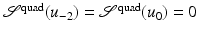 ; see also Fig. 3 for the landscape of
  . The non-convexity of
  with respect to y c can then be seen by considering convex combinations of y −2 and y 0. Since
 ![$$\mathcal{S}^{{\mathrm{quad}}}(u_{-1}) = 3/2 > 0$$” src=”/wp-content/uploads/2016/04/A183156_2_En_39_Chapter_IEq52.gif”></SPAN>, <SPAN id=IEq53 class=InlineEquation><IMG alt=$$\mathcal{S}^{{\mathrm{quad}}}$$ src=]() is not convex in y. Also note that y −1 is non-invertible and still has finite energy.
is not convex in y. Also note that y −1 is non-invertible and still has finite energy.
; see also Fig. 3 for the landscape of . The non-convexity of with respect to y c can then be seen by considering convex combinations of y −2 and y 0. Since 


Another serious drawback of both the energies  and
and  is that both yield finite energy for transformations that are not one-to-one; see Example 4. In addition, even for invertible transformations, the above regularization functionals do not explicitly control tissue compression and expansion; see Example 5. Thus, unlimited compression is performed, if sufficient reduction of the distance functional can be gained.
and is that both yield finite energy for transformations that are not one-to-one; see Example 4. In addition, even for invertible transformations, the above regularization functionals do not explicitly control tissue compression and expansion; see Example 5. Thus, unlimited compression is performed, if sufficient reduction of the distance functional can be gained.Example 4.
Consider the non-invertible trivial map  , with u(x) = −x and ∇u = −I. Clearly, V = 4E = −2I and
 ![$${{\mathcal{S}}^{{\mathrm{elas}}}}[u] = 4 {{\mathcal{S}}^{{\mathrm{quad}}}}[u] = (9\nu + 3\mu ){\mathrm{vol}}(\varOmega )$$](/wp-content/uploads/2016/04/A183156_2_En_39_Chapter_IEq59.gif) . These regularizers give thus finite values that depend only on the Lamé constants and the volume of the domain Ω.
. These regularizers give thus finite values that depend only on the Lamé constants and the volume of the domain Ω.
, with u(x) = −x and ∇u = −I. Clearly, V = 4E = −2I and . These regularizers give thus finite values that depend only on the Lamé constants and the volume of the domain Ω.Example 5.
For the sequence of transformations y (n)(x): = 2−n x, it follows u(x) = (2−n − 1)x and det∇y = 2−3n . For large n, this transformation heavily compresses volume. However, the components of ∇u are bounded below by − 1, showing that arbitrary compressions are not detected properly.
Hyperelastic Regularization Functionals
Motivated by these observations, a desirable property of regularization functionals is rapid growth to infinity for det∇y → 0+. In the Example 5, the Jacobian determinant is det∇y = 2−3n indicating that the volume of a reference domain goes rapidly to zero with growing n. Controlling compression and expansion to physically meaningful ranges has been a central theme in image registration; see, e.g., [34–36, 40, 58, 59].
Models for the so-called Ogden materials [4, 18] use an energy function that satisfies this important requirement,
![$$\displaystyle{ \mathcal{S}^{{\mathrm{Ogden}}}[y] =\int _{\varOmega }\frac{1} {2}\alpha _{\ell}\vert \nabla u\vert ^{2} +\ \alpha _{\text{a}}\|{\mathrm{cof}}\nabla y\|_{ F}^{2} +\alpha _{\text{v}}\ \psi _{ \text{O}}(\det \nabla y)dx, }$$](/wp-content/uploads/2016/04/A183156_2_En_39_Chapter_Equ13.gif)
with regularization a parameters 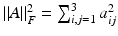 , and the convex penalty ψ O(v) = v 2 − logv. Note that this penalty ensures
 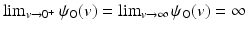 and thus gives infinite energy for non-invertible transformations. For small strains, linear elasticity is an approximation to this regularization functional; see [18]. For image registration, this energy was introduced first by Droske and Rumpf [23].
(10)
, and the convex penalty ψ O(v) = v 2 − logv. Note that this penalty ensures and thus gives infinite energy for non-invertible transformations. For small strains, linear elasticity is an approximation to this regularization functional; see [18]. For image registration, this energy was introduced first by Droske and Rumpf [23].While ensuring invertible transformations, the hyperelastic regularization functional (10) has drawbacks in the context of image registration: On the one hand, setting α a > 0 puts a bias towards transformations that reduce surface areas. On the other hand, setting α a = 0 prohibits the standard existence theory as presented in the next section. In addition, ψ O is not symmetric with respect to inversion, that is,  . Since det∇y −1 = (det∇y)−1 the value of the volume regularization term changes, when interchanging the role of template and reference image; see [17] for a discussion of the inverse consistency property.
. Since det∇y −1 = (det∇y)−1 the value of the volume regularization term changes, when interchanging the role of template and reference image; see [17] for a discussion of the inverse consistency property.To overcome these two drawbacks, the following hyperelastic regularizer as a slight modification of the Ogden regularizer (10) was introduced in [14],
![$$\displaystyle{\mathcal{S}^{{\mathrm{hyper}}}[y] =\int _{\varOmega }\frac{1} {2}\alpha _{\ell}(x)\vert \nabla u\vert ^{2} +\ \alpha _{\text{a}}(x)\phi _{\text{c}}({\mathrm{cof}}\nabla y) +\alpha _{\text{v}}(x)\ \psi (\det \nabla y)dx.}$$](/wp-content/uploads/2016/04/A183156_2_En_39_Chapter_Equd.gif) Making the regularization parameter spatially dependent is a small conceptual contribution with potentially big impact for many applications. The main idea is to replace ψ O by a convex penalty ψ, fulfilling the growth condition, and satisfying ψ(v) = ψ(1∕v). More precisely, the convex functions
Making the regularization parameter spatially dependent is a small conceptual contribution with potentially big impact for many applications. The main idea is to replace ψ O by a convex penalty ψ, fulfilling the growth condition, and satisfying ψ(v) = ψ(1∕v). More precisely, the convex functions
 were suggested in [14]. The penalty ϕ c is a convexification of the distance to orthogonal matrices and the penalty ψ(v) is essentially a polynomial of degree two, thus guaranteeing det∇y ∈ L 2, which is important in mass-preserving registration. If det∇y ∈ L 1 suffices, ψ can be replaced by its square root. Note that ϕ c is designed to avoid the preference for area shrinkage in (10). A convexification is needed for the existence theory, which makes ϕ c blind against shrinkage, allowing only penalization of area expansion.
Constraints
It is often beneficial to include additional prior knowledge or expectations on the wanted transformation into the model. Two case studies will show exemplarily how to restrict the set of admissible transformations. The first one is related to volume constraints [35, 36, 59] and the second one to local rigidity constraints [38, 65].
Volume-preserving constraints are particularly important in a setting such as monitoring tumor growth, where a change of volume due to the mathematical model can be critical. In addition, registration problems requiring highly nonlinear deformations, e.g., arising in abdominal or heart imaging, can be stabilized by restricting volume change to a certain class.
Constraining compression and expansion of volume has been a central topic in image registration over many years. Following [36], a formal description reads
:=\det \nabla y(x) \leq \kappa _{ M}(x)\mbox{ for }x \in \varOmega,}$$](/wp-content/uploads/2016/04/A183156_2_En_39_Chapter_Equf.gif) where κ m and κ M are given bounds. Volume preservation was enforced by using penalties, equality constraints such as
where κ m and κ M are given bounds. Volume preservation was enforced by using penalties, equality constraints such as  , or box constraints; see, e.g., [34–36, 40, 58, 59].
, or box constraints; see, e.g., [34–36, 40, 58, 59].Another example for image-based constraints is local rigidity. Local rigidity constraints can improve the model in applications in which images show bones or other objects that behave approximately rigidly, such as head-neck images, motion of prostate in the pelvis cage, or the modelling of joints. Rigidity on a subdomain Σ ⊂ Ω can be enforced by setting
![$$\displaystyle{\mathcal{C}^{{\mathrm{LR}}}[y,\varSigma ]:=\mathrm{ dist}(y,\mathcal{A}_{\mathrm{ rigid}}(\varSigma )\}) = 0;}$$](/wp-content/uploads/2016/04/A183156_2_En_39_Chapter_Equg.gif) see also Example 1. This formulation can be extended to multiple regions; see [38, 65].
see also Example 1. This formulation can be extended to multiple regions; see [38, 65].
Based on the discussion in [38], the Lagrangian framework has the advantage that the set Σ does not depend on y and thus does not need to be tracked; see [54] for a tracked Eulerian variant. Tracking the constrained regions may add discontinuities to the registration problem. In the case of local rigidity constraints, constraint elimination is an efficient option and results linear constraints. However, the Lagrangian framework involves det∇y in the computations of  and
and  ; see [38] for details.
and ; see [38] for details.Related Literature and Further Reading
Due to its many applications and influences from different scientific disciplines, it is impossible to give a complete overview of the field of image registration. Therefore this overview is restricted to some of the works, which were formative for the field or are relevant in the scope of this chapter. For general introductions to image registration, the reader is referred to the textbooks [33, 53, 55]. In addition, the development of the field has been documented in a series of review articles that appeared in the last two decades; see [11, 27, 31, 45, 52, 73].
A milestone for registration of images from different imaging techniques, or modalities, was the independent discovery of the mutual information distance functional by Viola and Wells [71] and Collignon et al. [19]. In this information theoretic approach, the reference and template images are discretized and interpreted as a sequence of grey values. The goal is to minimize the entropy of the joint distribution of both sequences. Due to its generality, mutual information distance measures can be used for a variety of image modalities. However, it is tailored to discrete sequences and thus the mutual information of two continuous images is not always well defined; see [42]. Furthermore, a local interpretation of the distance is impossible. To overcome these limitations, a morphological distance functional [23] and an approach based on normalized gradient fields [56] were derived for multimodal registration. Both approaches essentially use image gradients to align corresponding edges or level sets.
In addition to the already mentioned elastic and hyperelastic regularization functionals, another example is the fluid registration by Christensen [16]. The difference between fluids and elastic materials lies in the model for the inner force. In contrast to elastic materials, fluids have no memory about their reference state. Thus, the fluid registration scheme allows for large, nonlinear transformations while preserving continuity and smoothness. However, similar limitations arise from the fact that volume changes are not monitored directly.
It is well known that nonlinear registration schemes may fail if the geometrical difference between the images is too large. To overcome this, a preregistration with a rigid transformation model is usually employed. The above regularizers are, however, not invariant to rigid transformations. To overcome this limitation, the curvature regularization functional, based on second derivatives, was proposed [26, 43].
Similar to the linearized elastic regularization functional, fluidal or curvature regularized schemes fail to detect non-invertible transformations. As an alternative to hyperelastic schemes, the invertibility of the solution is to restrict the search for a plausible transformation to the set of diffeomorphisms as has been originally suggested by Trouvé in 1995 [69] and resulted in important works [3, 5, 70]. A transformation y is diffeomorphic, if y and y −1 exist and are continuously differentiable. The existence of an inverse transformation implies that diffeomorphisms are one-to-one. While invertibility is necessary in most problems, it is not always sufficient as the Example 5 indicates: for large n the size of the transformed domain has no physical meaning; see [55] for further discussions.
Image registration is closely related to the problem of determining optical flow, which is a velocity field associated with the motion of brightness pattern in an image sequence. First numerical schemes have been proposed by Horn and Schunck [48] and Lucas and Kanade [51] in 1981. In their original formulations, both approaches assume that a moving particle does not change its intensity. This gives one scalar constraint for each point. Hence, as image registration, determining the flow field is an under-determined problem. The under-determinedness is addressed differently by both approaches. The method by Horn and Schunck generates dense and globally smooth flow fields by adding a regularization energy. Lucas and Kanade, in contrast, suggest to smooth the image sequence and compute the flow locally without additional regularization. A detailed comparison and a combination of the benefits of both approaches is presented in [12].
There are many variants of optical flow techniques. For example, Brune replaced the brightness constancy by a mass-conservation constraint; see [13]. This gives the optical flow pendant to mass-preserving image registration schemes; see [30, 60, 61] and sections “Distance Functionals” and “Motion Correction of Cardiac PET”. Further, rigidity constraints have been enforced in optical flow settings in [50].
One difference between image registration and optical flow lies in the available data. In optical flow problems, motion is typically computed based on an image sequence. Thus, the problem is space and time dependent. If the time resolution of the image sequence is sufficiently fine, geometrical differences between successive frames can be assumed to be small and displacements can be linearized. In contrast to that, in image registration the goal is typically to compute one transformation that relates two images with typically substantial geometrical differences.
The problem of mass-preserving image registration is closely related to the famous Monge–Kantorovich problem of Optimal Mass Transport (OMT) [1, 6, 24, 49]. It consists of determining a transport plan to transform one density distribution into another. To this end, a functional measuring transport cost is minimized over all transformations that satisfy ![$$\mathcal{D}^{{\mathrm{MP}}}[y] = 0$$](/wp-content/uploads/2016/04/A183156_2_En_39_Chapter_IEq67.gif) in (7). A key ingredient is the definition of the cost functional which defines optimality. Clearly there is an analogy the cost functional in OMT and the regularization functional in mass-preserving image registration.
in (7). A key ingredient is the definition of the cost functional which defines optimality. Clearly there is an analogy the cost functional in OMT and the regularization functional in mass-preserving image registration.
in (7). A key ingredient is the definition of the cost functional which defines optimality. Clearly there is an analogy the cost functional in OMT and the regularization functional in mass-preserving image registration.3 Existence Theory of Hyperelastic Registration
The variational image registration problem (2) is ill-posed problem in the sense of Hadamard; see section “Ill-Posedness and Regularization” and [27, 55]. As Example 2 of a rotating disc suggests, uniqueness can in general not be expected. However, hyperelastic image registration has a sound existence theory which will be revisited in this section.
The main result of this section is the existence theorem for unconstrained hyperelastic image registration that includes all commonly used distance measures. It is further shown that solutions satisfy det∇y > 0, which is necessary in many applications. The theory is complicated due to the non-convexity of the determinant mapping as has been pointed out by Ciarlet [18, p.138f]. Using his notation F = ∇u: “The lack of convexity of the stored energy function with respect to the variable F is the root of a major difficulty in the mathematical analysis of the associated minimization problem.”
This section organizes as follows: A sketch of the existence proof is given in section “Sketch of an Existence Proof”. Formal definitions of involved function spaces, the set of admissible transformations, and the hyperelastic regularization functional  are given in section “Set of Admissible Transformations”. Finally, an existence result is shown in section “Existence Result for Unconstrained Image Registration”.
are given in section “Set of Admissible Transformations”. Finally, an existence result is shown in section “Existence Result for Unconstrained Image Registration”.Sketch of an Existence Proof
This section gives an overview of the existence theory of hyperelastic image registration problems. The goal is to outline the major steps, give intuition about their difficulties, and introduce the notation. The presentation is kept as informal as possible. The mentioned definitions, proofs, and theorems from variational calculus can be found, for instance, in [25, Ch. 8] or [18, 20].
The objective functional in (1) can also be written as an integral over a function  :
:
![$$\displaystyle{ \mathcal{J} [y] =\int _{\varOmega }f\big(x,y(x),\nabla y(x)\big)\ dx, }$$](/wp-content/uploads/2016/04/A183156_2_En_39_Chapter_Equ14.gif)
where the dependence on the template and reference images is hidden for brevity.
:(11)
In the following it is assumed that f is continuously differentiable and measurable in x. This is granted for the part related to the hyperelastic regularization functional. For the part related to the distance functional, this can be achieved by using a continuous image model  and
and  and careful design of
  .
.
and and careful design of .Typically,  is bounded below by a constant
 ![$$m:=\inf _{y}\mathcal{J} [y]$$](/wp-content/uploads/2016/04/A183156_2_En_39_Chapter_IEq74.gif) . The goal is to find a minimizer in a certain set of admissible transformations
. The goal is to find a minimizer in a certain set of admissible transformations  , which is a subset of a suitable Banach space X. Since X must be complete under Lebesgue norms, our generic choice is a Sobolev space
  , with p ≥ 1, rather than
  .
.
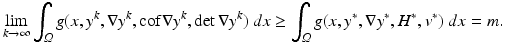
is bounded below by a constant . The goal is to find a minimizer in a certain set of admissible transformations , which is a subset of a suitable Banach space X. Since X must be complete under Lebesgue norms, our generic choice is a Sobolev space , with p ≥ 1, rather than .Existence of minimizers is shown in three steps. Firstly, a minimizing sequence  is constructed, that is, a sequence with
 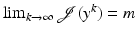 containing a convergent subsequence. Secondly, it is shown that its limit y ∗ is a minimizer of
  , in other words,
 ![$$\mathcal{J} [y^{{\ast}}] = m$$](/wp-content/uploads/2016/04/A183156_2_En_39_Chapter_IEq81.gif) . Finally, it is verified that y ∗ actually belongs to the admissible set
. Finally, it is verified that y ∗ actually belongs to the admissible set  .
.
is constructed, that is, a sequence with containing a convergent subsequence. Secondly, it is shown that its limit y ∗ is a minimizer of , in other words, . Finally, it is verified that y ∗ actually belongs to the admissible set .Key ingredients of the existence proof are coercivity and lower semicontinuity.
In a finite dimensional setting, the coercivity inequality
![$$\displaystyle{ \mathcal{J} [y] \geq C\ \|y\|_{X} + K\text{ for all }y \in \mathcal{A}\mbox{ and constants $C > 0$ and $K \in \mathbb{R}$}, }$$” src=”/wp-content/uploads/2016/04/A183156_2_En_39_Chapter_Equ15.gif”></DIV></DIV><br />
<DIV class=EquationNumber>(12)</DIV></DIV>guaranties that {<SPAN class=EmphasisTypeItalic>y</SPAN> <SUP><SPAN class=EmphasisTypeItalic>k</SPAN> </SUP>}<SUB> <SPAN class=EmphasisTypeItalic>k</SPAN> </SUB>lies in a bounded and closed set. From the lower semicontinuity it follows<br />
<DIV id=Equh class=Equation><br />
<DIV class=EquationContent><br />
<DIV class=MediaObject><IMG alt=](/wp-content/uploads/2016/04/A183156_2_En_39_Chapter_Equh.gif) and thus y ∗ is a minimizer. However,
and thus y ∗ is a minimizer. However,  is infinite dimensional. Hence, bounded and closed sets are in general not compact and the existence of a norm-convergent subsequence cannot be assumed. Thus, less strict definitions of convergence have to be used.
is infinite dimensional. Hence, bounded and closed sets are in general not compact and the existence of a norm-convergent subsequence cannot be assumed. Thus, less strict definitions of convergence have to be used.Note that  is reflexive for p > 1. For these cases, it can be shown that there exists a subsequence that converges in the weak topology, i.e., with respect to all continuous, linear functionals on
  . Consequently, if
  fulfills a coercivity condition (12), a bounded minimizing sequence can be constructed which yields weakly converging subsequence.
is reflexive for p > 1. For these cases, it can be shown that there exists a subsequence that converges in the weak topology, i.e., with respect to all continuous, linear functionals on . Consequently, if fulfills a coercivity condition (12), a bounded minimizing sequence can be constructed which yields weakly converging subsequence.The second part, namely showing that the weakly convergent sequence actually converges to a minimizer, is in general more involved. Lower continuity of  with respect to weak convergence typically requires convexity arguments. In many examples of variational calculus, the integrand f of
  is convex in ∇y. Thus, the integrand f can be bounded below by a linearization in the last argument around ∇y. Using the weak convergence of
  and noting that y k → y ∗ strongly in L 2 by a compact embedding, the linear term vanishes and lower semicontinuity follows; see Theorem 2.
with respect to weak convergence typically requires convexity arguments. In many examples of variational calculus, the integrand f of is convex in ∇y. Thus, the integrand f can be bounded below by a linearization in the last argument around ∇y. Using the weak convergence of and noting that y k → y ∗ strongly in L 2 by a compact embedding, the linear term vanishes and lower semicontinuity follows; see Theorem 2.When using hyperelastic regularization or mass-preserving distance functionals,  also depends on the Jacobian determinant det∇y. Thus, the dependence of f on ∇y is non-convex and further arguments are required to obtain lower semicontinuity. To overcome this complication, one can follow the strategy suggested by Ball [4]. The idea is to introduce a splitting in (y, cof∇y, det∇y) and show convergence of the sequence
 where the exponents q > 0 and r > 0 are appropriately chosen. A coercivity inequality in the ∥ ⋅ ∥ X -norm yields a weakly converging subsequence as outlined above. Extending f by additional arguments, it follows
 is measurable in x and continuously differentiable. Most importantly, g is convex in the last three arguments. Consequently, weak lower semicontinuity of
  in X can be shown, i.e.,
  implies
 To undo the splitting, the identifications H ∗ = cof∇y ∗ and v ∗ = det∇y ∗ must be shown. This is uncritical if y is sufficiently measurable, i.e., p is greater than the space dimension d. Note that p is also the degree of the polynomial det∇y. For hyperelastic regularization, it is possible to show existence under even weaker assumptions, i.e., for d = 3 and p = 2. Key is the identity
 It will be shown that H ∗ = cof∇y ∗ and v ∗ = det∇y ∗ for exponents q = 4 and r = 2; see Theorem 4.
also depends on the Jacobian determinant det∇y. Thus, the dependence of f on ∇y is non-convex and further arguments are required to obtain lower semicontinuity. To overcome this complication, one can follow the strategy suggested by Ball [4]. The idea is to introduce a splitting in (y, cof∇y, det∇y) and show convergence of the sequence in X can be shown, i.e., impliesA final note is related to the positivity of the determinant. To assure that the Jacobian determinant of a solution is strictly positive almost everywhere, sufficient growth of  is required, i.e.,
 ![$$\mathcal{J} [y] \rightarrow \infty $$](/wp-content/uploads/2016/04/A183156_2_En_39_Chapter_IEq94.gif) for det∇y → 0+. Note, that det∇y ∗ > 0 is not obvious. For example, k −1 → 0 although k −1 > 0 for all k.
for det∇y → 0+. Note, that det∇y ∗ > 0 is not obvious. For example, k −1 → 0 although k −1 > 0 for all k.
is required, i.e., for det∇y → 0+. Note, that det∇y ∗ > 0 is not obvious. For example, k −1 → 0 although k −1 > 0 for all k.Set of Admissible Transformations
As pointed out, regularization functionals involving det∇y considerably complicate existence theory due to the non-convexity of the determinant mapping. Thus, a careful choice of function spaces and the set of admissible transformations is important for the existence theory to be investigated in the next section. The goal of this section is to define the function spaces and the set of admissible transformations underlying the hyperelastic regularization functional (10).
To begin with, the problems arising from the non-convexity of the determinant are addressed. One technique to bypass this issue is a splitting into the transformation, cofactor and determinant and study existence of minimizing sequences in a product space. Here the product space
with the norm

is considered. The space X is reflexive and the norms are motivated by the fact that the penalty functions ϕ c and ψ presented in section “Hyperelastic Regularization Functionals” are essentially polynomials of degree four and two, respectively. The splitting is well defined for transformations in the set
![$$\displaystyle{ \mathcal{A}_{0}:= \left \{y:\ (y,{\mathrm{cof}}\nabla y,\det \nabla y) \in X,\ \det \nabla y > 0\ \text{a.e.}\right \}. }$$” src=”/wp-content/uploads/2016/04/A183156_2_En_39_Chapter_Equ19.gif”></DIV></DIV><br />
<DIV class=EquationNumber>(15)</DIV></DIV></DIV><br />
<DIV class=Para>To satisfy a coercivity inequality, boundedness of the overall transformation is required. In the standard theory of elasticity, this is typically achieved by imposing boundary conditions; see [<CITE><A href=]() 4, 18]. In the image registration literature, a number of conditions, for instance, Dirichlet, Neumann, or sliding boundary conditions were used; see [53].
4, 18]. In the image registration literature, a number of conditions, for instance, Dirichlet, Neumann, or sliding boundary conditions were used; see [53].
Get Clinical Tree app for offline access
(13)
(14)
Since finding boundary conditions that are meaningful for the application in mind often is difficult, the existence proof in section “Existence Result for Unconstrained Image Registration” is based on the following arguments. Recall that images are compactly supported in a domain Ω, which can be bounded by a constant  . Since images vanish outside Ω, reasonable displacements are also bounded by a constant only depending on Ω; see also discussions in [14, 58],
 For larger displacements, the distance functional is constant in y as the template image vanishes and thus no further reduction of the distance functional can be achieved. In this case, the regularization functional drives the optimization to a local minimum. Working with the supremum of y, however, complicates our analysis as the transformations in the non-reflexive space L ∞ . Therefore, an averaged version of a boundedness condition can be used:
. Since images vanish outside Ω, reasonable displacements are also bounded by a constant only depending on Ω; see also discussions in [14, 58],This leads to the following characterization of admissible transformations and definition of the hyperelastic regularization energy.
Definition 3 (Hyperelastic Regularization Functional).
Let  be a domain bounded by a constant M > 0,
 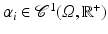 be regularization parameters with
 ![$$\alpha _{i}(x) \geq a_{i} > 0$$” src=”/wp-content/uploads/2016/04/A183156_2_En_39_Chapter_IEq98.gif”></SPAN> for all <SPAN class=EmphasisTypeItalic>x</SPAN> and <SPAN class=EmphasisTypeItalic>i</SPAN> = <SPAN class=EmphasisTypeItalic>l</SPAN>, <SPAN class=EmphasisTypeItalic>a</SPAN>, <SPAN class=EmphasisTypeItalic>v</SPAN>, and <SPAN id=IEq99 class=InlineEquation><IMG alt=$$\mathcal{A}_{0}$$ src=]() as in (15). The set of admissible transformations is
as in (15). The set of admissible transformations is
 Then the hyperelastic regularization functional is defined as
![$$\displaystyle{ \mathcal{S}^{{\mathrm{hyper}}}: \mathcal{A}\rightarrow \mathbb{R}^{+},\qquad \mathcal{S}^{{\mathrm{hyper}}}[y] = \mathcal{S}^{{\mathrm{length}}}[y] + \mathcal{S}^{{\mathrm{area}}}[y] + \mathcal{S}^{{\mathrm{vol}}}[y], }$$](/wp-content/uploads/2016/04/A183156_2_En_39_Chapter_Equ20.gif)
with
![$$\displaystyle\begin{array}{rcl} \mathcal{S}^{{\mathrm{length}}}[y]& = & \int _{\varOmega }\alpha _{\ell}(x)\ \vert \nabla u(x)\vert ^{2}dx,{}\end{array}$$](/wp-content/uploads/2016/04/A183156_2_En_39_Chapter_Equ21.gif)
![$$\displaystyle\begin{array}{rcl} \mathcal{S}^{{\mathrm{area}}}[y]& = & \int _{\varOmega }\alpha _{\text{a}}(x)\ \phi _{\text{c}}({\mathrm{cof}}\nabla y(x))dx,{}\end{array}$$](/wp-content/uploads/2016/04/A183156_2_En_39_Chapter_Equ22.gif)


be a domain bounded by a constant M > 0, be regularization parameters with (16)
(17)
(18)
Related posts:

Stay updated, free articles. Join our Telegram channel
Full access? Get Clinical Tree
