Imaging Parameters
Mark Doyle
OVERVIEW
A common starting point for many topic areas in magnetic resonance imaging (MRI) is the phenomenon of k-space. K-space is essentially the “raw material” from which magnetic resonance (MR) images are derived, that is, it is the signal space. There are a number of important options in the scanner interface that directly affect the manner in which k-space is acquired. These features or options can have a dramatic impact on imaging time, quality, and contrast. Here we will discuss scanner interface features in terms of k-space.
K-SPACE PROPERTIES
To produce a cardiac image series, we have to balance spatial and temporal resolution features. These can be distributed in a variety of ways, each affecting a different aspect of image quality. Each k-space property has a direct impact on multiple aspects of image quality.
Dimensions of k-Space
When considering a k-space matrix, “conventional” MRI acquisition methods essentially compile k-space one line at a time. The image is produced by performing the Fourier transform operation on the completed k-space data. Often, the Fourier transform is referred to as the fast Fourier transform (FFT), in reference to a particularly efficient mathematical algorithm that is used to perform the operation. One relationship linking the k-space data and the image data is that the dimensions of k-space are the same as the image, for example, a square k-space data set with 128 × 128 data points generates an image that is square, also with 128 × 128, picture elements, or pixels. In this respect there is a one-to-one correspondence between the number of k-space points and the number of image points.
Temporal Blur
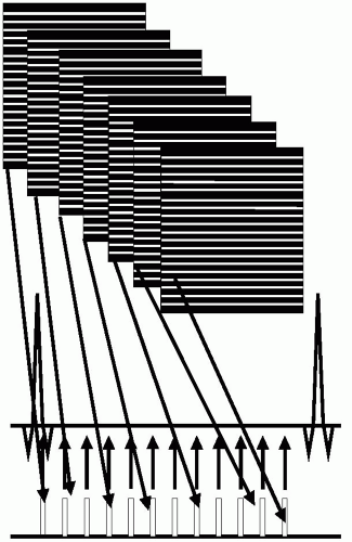
In cardiac imaging, each image at each cardiac phase is formed from a k-space data set, typically generated as a series of lines, (see Fig. 21-1). For breath-hold approaches, cine images are typically acquired in a “segmented” or “turbo” manner such that each cardiac view is rapidly compiled by acquiring a group of lines or views per segment (VPS), during successive cardiac cycles, (see Fig. 21-2). In a segmented scan, data for each cardiac phase are acquired by a short “string” of acquisitions (e.g., eight views). Each element of the segment has a duration, Td, and thereby the duration of each segment, Tseg, is given by Td multiplied by the number of segments (in this example, Tseg = 7 × Td). It is apparent that for a cardiac image series, one of the determinants of scan time is the VPS factor that is used. For example, consider a matrix of 256 × 256 being acquired at a rate of one line per cardiac cycle. At this rate, the scan time required extends over 256 heartbeats (˜4 minutes, depending on heart rate). By increasing the VPS beyond 1, the scan time is reduced in a linear manner:
The advantage of using a high VPS factor is that scan time is dramatically reduced. However, one disadvantage of selecting too high a VPS value is that temporal blur may result within the cardiac cycle. Consider the example where the repetition time (TR) is 4 milliseconds; the resulting segmentation time (Tseg) increases with increasing VPS values:
Therefore, as the VPS increases, the degree of temporal blur associated with each cardiac view also increases. Further, when employing data segmentation, the number of cardiac phases that can be fitted into each cardiac cycle is reduced in direct proportion to the VPS value. For example, consider a patient with a heartbeat interval of 1,000 milliseconds. As the VPS value increases, the number of intervals in which data can be acquired decreases:
VPS = 8, segment time = 32 milliseconds, number of cardiac phases = 1,000/32 = 31
VPS = 16, segment time = 64 milliseconds, number of cardiac phases = 1,000/64 = 15
VPS = 20, segment time = 80 milliseconds, number of cardiac phases = 1,000/80 = 12
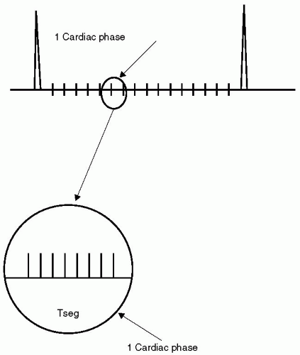 FIGURE 21-2 In cardiovascular magnetic resonance (CMR), scan time is reduced by employing segmentation. In a segmented scan, each cardiac phase is acquired by a short “string” of acquisitions (eight views in this example). The scan time is reduced by a factor equal to the segmentation factor. |
View Sharing
A processing option that confounds the simple calculations in the preceding text is “view sharing”. View sharing can be used to increase the temporal resolution within the cardiac cycle, irrespective of the VPS value selected! Essentially, the view sharing option allows generation of images at intermediate cardiac phases, that is, images are generated in between each directly acquired segmented data set (see Fig. 21-3). In view sharing, k-space data from two directly acquired adjacent cardiac phases are combined to construct an intermediate k-space data set, for example, in the VPS 7 example, the last four views of the cardiac phase number 5 are combined with the first three views of data from cardiac phase number 6 to form cardiac phase 5.5, and so on. In this example, the number of cardiac phases that are represented is almost doubled. For example, if 15 phases are directly acquired, 29 (i.e., 2 × n – 1) phases may be generated by view-sharing data. On some scanners, the number of views represented in the final cardiac series can be set almost arbitrarily when more general data interpolation and k-space combination approaches are used. Therefore, caution should be exercised when


Stay updated, free articles. Join our Telegram channel

Full access? Get Clinical Tree


