Intracranial Hemorrhage
Scott W. Atlas
Keith R. Thulborn
The initial recognition of intracranial hemorrhage has crucial and immediate implications for further diagnostic workup, clinical management, and ultimately patient outcome. Although the basic signal intensity of evolving intracranial hemorrhage has become widely known, new pulse sequences and higher scanner field strengths continue to emerge, and these have added even more importance to understanding the biological variables (Table 10.1) and technical operator-dependent imaging parameters (Table 10.2) that alter the magnetic resonance imaging (MRI) patterns when hemorrhage is present.
Although these complex patterns make MR interpretation challenging, they also make hemorrhage an excellent vehicle for demonstrating the principles underlying MR contrast. As in past editions, this chapter goes beyond the simple pattern recognition style of radiologic diagnosis to a more detailed description of the physics and biochemistry underlying the various MR phenomena illustrated during the evolution of cerebral hematomas. Once understood, these principles can be used to understand the signal characteristics of many other entities. This allows the radiologist to put forth more specific diagnoses, instead of long lists of possibilities that often add little value to the referring clinical team.
Beyond the initial diagnosis, the radiologist needs to be cognizant of several specific goals when interpreting brain MR studies in the search for hemorrhage (Table 10.3). These goals center on recognizing key neuroanatomic findings that influence patient management and direct further workup. Fundamental principles of neuroradiologic diagnosis, separate from the consideration of MR signal intensities, must be used to assist the clinician in providing optimal patient care. Localization of the hemorrhage to the intraaxial or extraaxial space is central to assessing etiology and to the initiation of treatment. If blood is extraaxial, it is important to specify whether it is subdural or epidural. If hemorrhage is intraaxial, it must be determined whether it originated in the subarachnoid space rather than the parenchyma. In certain instances, intracranial hemorrhage can be multi-compartmental, so familiarity with etiologies for these cases is essential for appropriate tailoring of further workup (see later sections in this chapter).
TABLE 10.1 Physiologic Factors Influencing Magnetic Resonance Appearance of Hematomas | |||||||||||
|---|---|---|---|---|---|---|---|---|---|---|---|
|
Once the basic neuroanatomic features are assessed, more sophisticated diagnoses that are crucial to patient management often can be gleaned from MR on detailed analysis of signal intensity. In clinical settings, it should be common for MR to be recommended after an acute intracerebral hemorrhage is diagnosed on computed tomography (CT) because the etiology of the hemorrhage can be discerned by using the information that is uniquely available from MR studies. This third level of image interpretation—the analysis of the subtle secondary findings on MR associated with hemorrhage—can be extremely important to the ultimate diagnosis of etiology and workup.
The conceptual framework for understanding the MR appearance of intracerebral hematomas has been summarized in multiple reviews (1,2,3,4,5) based on in vitro studies, animal models, and clinical observations (2,6,7,8,9,10,11,12,13,14,15,16,17,18,19). As put forth in the original descriptive model (12), the two most important biophysical properties in the generation of MR signal intensity patterns seen in evolving intracranial hematomas are the paramagnetic effects of iron associated with the changing oxygenation states of hemoglobin and the integrity of red blood cell (RBC) membranes that, when intact, compartmentalize the paramagnetic iron. Iron clearly plays a dominant role, even more so now that higher-field scanners are in practice (20,21), because its magnetic properties vary as its biochemical form, oxidation state, and spatial distribution change. Investigations have also supported the role of RBC membrane integrity in MR features of hematomas (22). Other pathophysiologic processes, including findings relating to the presence of an underlying neoplasm (i.e., persistent hypoxia, lack of integrity of the blood–brain barrier, alteration of the degree of edema, recurrent bleeding, bleeding into cystic or necrotic regions), coagulopathy, and nonparamagnetic protein concentration contribute to signal intensity patterns on these images. RBC volume (23), thrombus formation, and clot retraction (24) may be of some importance. Structural
alterations, such as cavitation and hemoglobin resorption or degradation, become significant as the more acute processes of iron metabolism and edema decrease in importance during hematoma evolution.
alterations, such as cavitation and hemoglobin resorption or degradation, become significant as the more acute processes of iron metabolism and edema decrease in importance during hematoma evolution.
TABLE 10.2 Operator-Dependent Factors Influencing Magnetic Resonance Appearance of Hematomas | ||||
|---|---|---|---|---|
|
TABLE 10.3 Goals of Imaging Hemorrhage | |||||
|---|---|---|---|---|---|
|
This chapter reviews the physicochemical principles of the magnetic properties of matter and their applications to biological systems, discusses the biochemical pathways of iron metabolism and water balance in resolving intracerebral hematomas, and presents a qualitative scheme for relating these biochemical processes to the relaxation phenomena underlying signal contrast observed in MR images of hemorrhage. Factors most important to the intensity patterns in evolving intracranial hematomas are stressed. More recent concepts concerning the use of MR in the diagnosis and characterization of intra- and extraaxial hemorrhages, including subarachnoid hemorrhage (SAH), are included. When important, the effect of field strength is emphasized. MR features suggestive of specific clinical etiologies of intracranial hemorrhage are also discussed. MR mimics of hemorrhage, based on signal intensity patterns, will be illustrated.
Origin of Magnetism
A magnetic field is generated by a moving electric charge (25). The strength of the magnetic field is determined by the size of the electric charge and by its momentum. The magnetic field generated by the unit charge is termed a magnetic dipole. An electron confined to an atomic orbital represents a moving charge with both orbital angular momentum and spin angular momentum. Each angular momentum of the electron (i.e., orbital and spin) generates a magnetic field. Because the nucleus also possesses an electric charge and may have nonzero spin angular momentum (spin quantum number 0, 1/2, 3/2, …), it may also generate a magnetic field. However, because the magnetic moment of any charged particle is inversely proportional to its mass, and the mass of the nucleus is three orders of magnitude greater than that of the electron, the contribution of the nucleus to the magnetic properties of the atom is much less than that of the electrons. Hence, although nuclear magnetic interactions occur and nuclear magnetization is the origin of the signal used to construct the MR image, the magnetic properties of tissue are determined chiefly by the electronic configuration of the atoms and molecules.
The two major types of magnetic properties of matter most relevant to a discussion of human biological systems are diamagnetism and paramagnetism. These concepts are first reviewed in terms of the different electronic configurations of the atoms and molecules that make up the constitutive material. Other magnetic properties of matter are discussed in detail elsewhere (5) and are reviewed here briefly.
Diamagnetism
Most biological materials consist of elements such as carbon, oxygen, and hydrogen, in which the electrons are paired in atomic and molecular orbitals. The pairing of electrons with opposite spin angular momentum minimizes the energy state of the electrostatic and magnetic interactions of closely placed identical charges (i.e., the electrons). In the paired condition, the net spin angular momentum of electrons is zero (i.e., there is no net magnetic moment). However, the paired electrons still have orbital angular momentum, constituting charges circulating in a confined orbital. If such a current loop is placed in an applied magnetic field, Lenz’ law states that this current loop (i.e., the electrons) generates a magnetic field opposing the applied magnetic field in vector direction (Fig. 10.1A). This reduces the magnitude of the local magnetic field within the material below that of the original applied magnetic field. Materials that reduce the magnitude of an applied magnetic
field are termed diamagnetic; greater than 99% of human tissue is diamagnetic.
field are termed diamagnetic; greater than 99% of human tissue is diamagnetic.
 FIGURE 10.1 A: Diamagnetism. B: Paramagnetism. C: Antiferromagnetism. D: Ferromagnetism. |
Paramagnetism
Biological substances containing atomic or molecular structures with unpaired electrons have magnetic properties dominated by those unpaired electrons, due to the resultant magnetic dipole arising from the electronic spin angular momentum. Iron, in its ferrous and ferric oxidation states, is an important example of a naturally occurring substance in which the number of unpaired electrons varies with the biochemical state of the metal ion. If the magnetic dipoles of a collection of atoms or molecules are widely separated and randomly oriented in space, such that the unpaired orbital electrons on different atoms cannot interact, then the total magnetic field from that collection is zero. However, individual electronic magnetic dipoles can respond to an applied magnetic field by aligning in a parallel or antiparallel manner to that field, according to quantum mechanical requirements of the two–energy-state system for spin particles. The distribution of electrons between the two energy states is governed by the Boltzmann distribution. At physiologic temperatures, more electrons align parallel to the applied field, resulting in an enhancement (i.e., an increase in magnitude) of that applied field (Fig. 10.1B). This phenomenon is analogous to the alignment of nuclear spins in the nuclear magnetic resonance (NMR) experiment. Materials that have no intrinsic magnetic field in the absence of an applied magnetic field but augment an applied magnetic field on exposure to it are termed paramagnetic. Naturally occurring paramagnetic substances include copper, iron, and manganese.
Antiferromagnetism, Ferromagnetism, and Superparamagnetism
Some biologically important materials, such as the ferric oxyhydroxide crystalline structure of ferritin and hemosiderin (two forms of iron storage substances), consist of closely packed ensembles of atoms with unpaired electrons and demonstrate yet another type of magnetic behavior that is relevant to MR. In such substances, unpaired electrons of neighboring atoms interact to minimize net magnetic forces. Resultant magnetic forces that produce “preferred” patterns of spin alignments are termed exchange forces.
If unpaired electrons of pairs of adjacent atoms align with opposing spins, magnetic forces are minimized. In an applied magnetic field, spin pairing must be actively disrupted if individual electronic spins are to realign with the applied magnetic field. Because this disruption requires energy, the overall response of the material to the applied field (i.e., the degree of augmentation of the applied field) is less than that of a paramagnetic substance. Note that the net (effective) magnetic field is still increased in comparison with the magnitude of the original applied field (Fig. 10.1C). Materials exhibiting this behavior are termed antiferromagnetic. The alignment pattern in antiferromagnetic substances can be disrupted if the thermal energy is increased, and initially the response to an applied field is enhanced as the temperature is increased. Above a critical temperature, known as the Néel temperature, adjacent spin pairing is disrupted, and the antiferromagnetic substance becomes paramagnetic.
If the unpaired electrons of a group of atoms in a crystal interact to align in domains (termed Weiss domains), each domain has its own net magnetic field. Adjacent Weiss domains can then interact via these magnetic fields to minimize the resultant magnetic field outside of the material. If that material is immersed in a high magnetic field, domains respond to both the applied field and neighboring domain fields to enhance markedly the overall field (Fig. 10.1D). Such materials possess a magnetic field even in the absence of an applied magnetic field and are termed ferromagnetic.
As the ferromagnetic crystal is reduced in size to that of a single domain, this single-domain equivalent particle has a net magnetic dipole equivalent to that of a single domain. If a collection of such single-domain particles is free to rotate in an applied magnetic field on a time scale that is shorter than the observation time, the magnetic dipoles behave as expected for paramagnetism (discussed earlier). However, the larger magnetic moment of the particle (because it is a domain or group of atoms acting as one) produces a greater enhancement of the applied magnetic field compared with paramagnetic substances. Such particles are termed superparamagnetic (26,27,28). Superparamagnetic materials do not retain their magnetic field when removed from an applied field.
If the size of the particles (which normally contain many domains) is reduced below the size of a single domain, the aligning exchange forces and disaligning thermal forces become comparable. Assuming that the time scale of the observation is longer than the switching rate of the equilibrium between the aligned and disordered states, then the magnetic properties of the particles depend on the temperature–volume relationships, which determine the switching frequency. An aggregate of such particles behaves paramagnetically but with a greater magnetic dipole than if no domain formed at all and thus is termed supermagnetic (25).
Antiferrimagnetism and Ferrimagnetism
When a crystal lattice is composed of two different substances, the lattice symmetry can be such that the resultant structure allows exchange forces between atoms of the two substances to operate separately. This behavior resembles two separate crystals occupying the same space. The exchange forces may allow individual opposition (antiferrimagnetism) or group opposition (ferrimagnetism).
Magnetic Susceptibility
Any material, when placed into a constant magnetic field, responds by generating its own magnetic field. The magnetic susceptibility of a substance (or tissue) describes this magnetic response. The induced magnetic field has two important characteristics: a magnitude and a vector direction. Materials can be categorized based on their induced fields (i.e., based on their magnetic susceptibilities) (Table 10.4).
Diamagnetic materials respond to an applied field with a very weak induced field (approximately 10−6 × the magnitude of the applied field) and in a vector direction that opposes that of the applied field. Paramagnetic materials have a larger induced field (approximately 10−2 to 10−4 × the magnitude of the applied field), which is in the same vector direction as the applied field. Superparamagnetic and ferromagnetic materials generate a very large induced field, equal to or even greater than the applied field, and, as with paramagnetic substances, the induced field is in the same vector direction as the applied field.
The tissue interaction with the static magnetic field B0 to produce magnetization m, which either reduces (diamagnetism)
or enhances (paramagnetism, antiferromagnetism, ferromagnetism, superparamagnetism) the effective magnetic field Beff within the material (note that the magnetization m refers to the effects of electronic configurations, not to the nuclear magnetization M measured in the NMR experiment), can be quantified in terms of the magnetic susceptibility χ of the material, where
or enhances (paramagnetism, antiferromagnetism, ferromagnetism, superparamagnetism) the effective magnetic field Beff within the material (note that the magnetization m refers to the effects of electronic configurations, not to the nuclear magnetization M measured in the NMR experiment), can be quantified in terms of the magnetic susceptibility χ of the material, where
where
TABLE 10.4 Magnetic Susceptibility Based on Characteristics of the Induced Magnetic Field | |||||||||||||||
|---|---|---|---|---|---|---|---|---|---|---|---|---|---|---|---|
|
 FIGURE 10.2 The effective magnetic field Beff is modified from the applied magnetic field B0 by the presence of tissue, depending on whether it is diamagnetic (χ < 0) or paramagnetic (χ < 0). The boundary between these regions has a gradient in Beff that functions as an apparent fluctuating magnetic field bz when spins diffuse across the boundary. Thus diffusion causes Mxy relaxation characterized by T2*. Because no fluctuating fields occur along bx or by, Mz and, therefore, T1 are unaltered. |
Thus, χ < 0 for diamagnetic materials, χ < 0 for paramagnetic materials, and χ = 0 for a vacuum.
When placed into the static magnetic field of the imaging magnet, therefore, tissues of different magnetic susceptibilities establish different effective local magnetic fields (Fig. 10.2). Consequently, when there are two adjacent regions of differing magnetic susceptibilities in the imaging volume, there are actually two adjacent regions of differing magnetic fields (Fig. 10.2). Gradients, or differences, in magnetic susceptibility χ could be thought of as equivalent to magnetic field inhomogeneities. The response of the nuclear magnetization measured in the MR image is altered dramatically by the different stages of iron metabolism found within an evolving hematoma due to their differences in magnetic susceptibility.
MR Contrast
Most clinical MR images are based on the nuclear spin system of hydrogen (I = 1/2), referred to simply as protons. The proton is intrinsically the most sensitive nucleus for MR and occurs in the highest concentration in the human body, given the abundance of water in human tissue. The protons have charge and spin and therefore behave as a magnetic dipole, as discussed for electrons earlier. As such, they respond to other magnetic fields, such as applied external magnetic fields, and to other local dipole fields produced by adjacent nuclei with nonzero spin and unpaired electrons. Image contrast is the difference in signal intensity arising from different regions of the object. If two regions have different magnetic environments, signal intensities from each region will be different and contrast will be observed. The nature of interactions between the magnetic environment and the proton spin system is discussed in terms of the MR process.
Relaxation Mechanisms in Hemorrhage
For diamagnetic tissues, the most important relaxation mechanism accounting for both longitudinal and transverse relaxations is attributed to proton–proton dipole–dipole interactions (27,29). Other mechanisms, scalar spin coupling, chemical shift anisotropy, quadrupolar, and spin–rotational effects, are usually less important in proton MR and are described elsewhere (30,29,31). The image contrast in hemorrhage requires discussion of two effects of nondiamagnetic substances. These are considered under relaxivity and susceptibility effects. A third process of exchange is discussed separately.
Relaxivity Effects
The rotational and translational diffusion of water molecules in biological systems occur on a time scale that produces an isotropically fluctuating magnetic field in the range of the Larmor frequencies for protons at current imaging field strengths. If the water molecules are able to approach a paramagnetic center, then magnetic interactions between the nuclear magnetic dipoles of the water (protons) and the magnetic dipoles of the paramagnetic centers (unpaired electrons) allow efficient energy exchange to occur. This interaction results in relaxation of the water proton to its magnetic equilibrium state (32). The phenomenologic equation for such intermolecular proton–electron dipole–dipole interactions with a paramagnetic agent, P, in bulk solution is given as
where
and i = 1, 2; R is the relaxivity constant (s−1 mM−1); and [P] is the concentration (mM) of the paramagnetic substance P. Here, 1/Ti(dia) is the relaxation rate due to diamagnetic relaxation processes and 1/Ti(para) is the relaxation rate in the presence of the paramagnetic species. In the presence of a suitable paramagnetic substance, the paramagnetic term dominates over the diamagnetic term in Equation 3. The same equation applies for both longitudinal and transverse relaxation. Because T1 is generally longer than T2 in biological systems, 1/T1 is smaller than 1/T2 and so the constant term R[P] contributes a greater proportion to the longitudinal relaxation rate (1/T1) than to the transverse relaxation rate (1/T2). The implication for MR is that the relaxivity effects attributed to dipole–dipole interactions with paramagnetic substances are detected with greater sensitivity on T1-weighted (short repetition time/echo time [TR/TE]) images than on T2-weighted (long TR/TE) images.
The contributions of “inner-sphere” (ligand exchange in which water molecules are in the first coordination sphere of P) and “outer-sphere” (diffusion with close approach of water near but without coordination to P) effects to paramagnetic relaxation rates can be further analyzed by the more mechanistic Solomon–Bloembergen equations, which are presented in detail elsewhere (34). It should be noted that application of Equation 3 to biological systems as complex as cerebral hematomas can only be approximate because of the heterogeneity in type and distribution of the various paramagnetic substances involved.
The strength of the dipole–dipole interaction between water and paramagnetic substances depends on several factors (Table 10.5): the number of unpaired electrons in the paramagnetic material (which, in turn, determines the magnetic moment), the concentration of the paramagnetic substance, the
electron spin relaxation rate, and, perhaps most relevant to the clinical images, the distance between the (potentially) interacting dipoles (interdipole distance).
electron spin relaxation rate, and, perhaps most relevant to the clinical images, the distance between the (potentially) interacting dipoles (interdipole distance).
TABLE 10.5 Factors Affecting Strength of Proton–Electron Dipole–Dipole (PEDD) Interaction | ||||
|---|---|---|---|---|
|
In fact, the strength of the dipolar interaction is proportional to the inverse sixth power of the interdipole distance (Fig. 10.3). The implication of this geographic restriction on the strength of relaxation enhancement is profound when one considers the MR intensity pattern in acute hematomas. When the water proton is unable to approximate close enough to the paramagnetic center (i.e., the unpaired electrons of deoxyhemoglobin), no dipole–dipole magnetic interaction, and therefore no relaxation enhancement, occurs by relaxivity mechanisms. This failure of interaction can be ascribed to the quaternary structure of deoxyhemoglobin (Fig. 10.4) (33). Therefore, even though deoxyhemoglobin is clearly paramagnetic, the acute hematoma is not hyperintense on T1-weighted images. After the acute event, when deoxyhemoglobin undergoes conversion to methemoglobin, conformational changes in the hemoglobin molecule–iron complex result in accessibility of the water proton to the unpaired electrons of iron in methemoglobin (Fig. 10.4) (33) and dipolar relaxation enhancement follows, resulting in the typical high intensity of methemoglobin in subacute and chronic hematomas.
Susceptibility Effects
As can be seen from Equation 3, dipole–dipole relaxation mechanisms affect both T1 and T2 (although not necessarily equally). This is because the fluctuating magnetic field of a randomly tumbling paramagnetic center is isotropic, operating along the x, y, and z axes. Magnetic susceptibility–induced relaxation, in contrast, does not affect both T1 and T2. This selective T2 relaxation enhancement can be understood by considering the precise mechanisms involved in generating magnetic susceptibility effects. There are two types of static magnetic fields that are highly anisotropic, operating only in the direction of the main field B0: inhomogeneities in B0 due to magnet imperfections
and magnetic susceptibility–induced field variations Beff. If the inhomogeneities in Beff are large over the dimensions of the voxel, the field variations produce dispersion in frequencies within the voxel, leading to rapid loss of transverse magnetization (this has also been described as loss of phase coherence of spins within that voxel). The combination of this loss of transverse magnetization from B0 inhomogeneities with dipole–dipole relaxation mechanisms is characterized by a combined relaxation time termed T2*. (Note that T2* refers to total transverse relaxation and can be described by the following equation:
and magnetic susceptibility–induced field variations Beff. If the inhomogeneities in Beff are large over the dimensions of the voxel, the field variations produce dispersion in frequencies within the voxel, leading to rapid loss of transverse magnetization (this has also been described as loss of phase coherence of spins within that voxel). The combination of this loss of transverse magnetization from B0 inhomogeneities with dipole–dipole relaxation mechanisms is characterized by a combined relaxation time termed T2*. (Note that T2* refers to total transverse relaxation and can be described by the following equation:
where T2 equals the transverse relaxation induced by spin–spin interactions, T2″ equals the transverse relaxation from B0 inhomogeneities, and T2′ equals the transverse relaxation related to susceptibility gradient–induced field inhomogeneities.) Spin-echo imaging minimizes the effects of static magnetic field variations (field inhomogeneities) with the use of the 180-degree refocusing RF pulse. In fact, this recovery of signal loss from field inhomogeneity is probably the major reason for the success of the spin-echo technique in imaging. Conversely, reversal of the readout gradient in the absence of a 180-degree RF pulse, which is used in gradient-echo imaging for generation of the echo, does not compensate for signal loss due to field inhomogeneities. As a consequence of the gradient-echo technique, gradient-echo imaging is extremely sensitive to field inhomogeneities, a feature that assumes greater importance at lower field strengths (33).
 FIGURE 10.3 Proton–electron dipole–dipole interaction schematic. The magnetic movement μ of the unpaired electron (e−) in the paramagnetic center is much larger (approximately 700 times) than that of the water protons (p+), as denoted by the larger arrow of the e−. The distance between the dipoles strongly influences the strength of the interaction (see text). The longer spirals imply stronger interactions at shorter distances between dipoles. |
 FIGURE 10.4 Structure of hemoglobin complex in various stages of evolving hemorrhage. A: Oxyhemoglobin. B: Deoxyhemoglobin. C: Methemoglobin. Note that iron (Fe) is nearly within the same plane as the atoms comprising the porphyrin ring (dark color) in the oxyhemoglobin (A) molecule. On deoxygenation, there is a subtle alteration in the position of Fe to become positioned outside of the porphyrin plane (B), which prevents access to water. In the methemoglobin state (C), note that the Fe is now positioned again nearly within the plane of the porphyrin ring, allowing close approximation by water (W). (Courtesy of Dr. Peter Janick, Philadelphia, PA, as modified from Dickerson RE, Geis I. Hemoglobin: Structure, Function, Evolution, and Pathology. Menlo Park, CA: Benjamin Cummings; 1983, with permission.) |
An additional cause of phase dispersion–induced signal loss distinct from that due to static field variations (as described earlier) relates to what can be considered time-varying magnetic field changes. The molecular diffusion of water that occurs through regions of variable Beff during TE (time between the 90-degree RF pulse and echo) produces frequency variations (Equation 2) and concomitant loss of phase coherence in the transverse plane resulting in signal loss in Mxy. The local fields experienced by the moving spins over the time of diffusion, although the fields are static, are analogous to a situation in which spins are stationary and change over that same period of time. In effect, then, the field can be considered to be varying over the time of spin diffusion. Note that this loss of signal is not recovered by the 180-degree RF pulse of the spin-echo sequence, so, in fact, both conventional spin-echo imaging and gradient-echo techniques are sensitive to this cause of hypointensity. This effect becomes more apparent as the TE exceeds the diffusional correlation time (time for a proton to move from one position to another position). Spins diffusing in the x–y plane experience these variations in Beff as a fluctuating magnetic field along bz, with resultant enhancement of transverse, but not longitudinal, relaxation (Fig. 10.2) (hence the term selective T2 shortening). This effect is well known in NMR spectroscopy (29), where a known magnetic field gradient G can be applied to a sample to measure the diffusion coefficient D of protons through a solvent. The signal intensity S for a Hahn spin echo at TE is given as
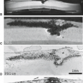
Magnetic susceptibility differences due to compartmentalization of paramagnetic species (e.g., iron) have a great effect on the signal intensity of evolving hematomas on T2 images. This compartmentalization is due to the presence of intact RBC membranes in early hematomas. Recent analysis of apparent diffusion coefficients from diffusion MR in clinical hematomas (22) supported this concept by documenting that water diffusion is significantly and equally restricted in intracranial hematomas with signal patterns consistent with intracellular oxyhemoglobin, intracellular deoxyhemoglobin, and intracellular methemoglobin as compared with hematomas containing extracellular methemoglobin (Fig. 10.5). Differences in susceptibilities between, for example, compartmentalized paramagnetic deoxyhemoglobin within an RBC and diamagnetic water can result in significant T2 relaxation if sufficient diffusion is permitted to occur during the imaging sequence (Fig. 10.6). Such effects cause marked signal loss in acute hematomas on long-TR/TE (T2-weighted) MR images without similar degrees of signal loss on either long-TR/short-TE (proton density–weighted) or short-TR/short-TE (T1-weighted) MR images. It has also been shown (35) that the use of prolonged interecho intervals (τcpmg) results in shortening of the effective T2, again by allowing more diffusion of water protons through areas of differing magnetic fields. The clinical importance of understanding this diffusion-related mechanism of T2 shortening is clear when one considers the clinical situation of attempting to depict acute (or chronic) hemorrhage on low–field-strength systems. To maximize the hypointensity on low–field-strength scanners, the long-TR protocol should include long TE with very long τcpmg. Indeed, the strength of this T2-shortening mechanism is related to several factors (Table 10.6).
Exchange Processes
Changes in the (nonparamagnetic) protein content within the hematoma also evolve as clot formation, clot contraction, and necrosis occur. From in vitro studies (36,37,38), increasing protein concentration would be expected to promote T1 and T2 relaxation rates. It is possible that the exchange of water between bulk and protein-bound (hydration layer) phases may be a significant contributor to proton relaxation in some situations of hemorrhage, especially on low-field scanners, where paramagnetic susceptibility mechanisms are not nearly as prominent as on high-field imagers. In fact, the lack of susceptibility-induced relaxation effects accounts for the lack of marked hypointensity (and therefore the lack of ability to detect with certainty) in most acute hematomas at low field.
Investigators demonstrated that changes in RBC volumes may be responsible for some of the changes in T2 relaxation rates in hematomas (23). With shrinkage of RBCs due to decreases in intracellular water, it has been shown that T2 can decrease significantly in in vitro studies of blood clots. This relaxation rate increase is probably related to protein concentration–dependent changes in the correlation time (a viscosity effect) (39), but further work needs to be done to clarify the significance of this mechanism in the in vivo hematoma.
Clark et al. (24) attempted to quantify the effects of deoxygenation, protein (hematocrit), clot formation, and clot retraction in generating signal intensity changes of acute hematomas. In their study, it was apparent that the contributions of fibrin clot formation and clot retraction to T2 shortening were minimal (less than 2% combined). Furthermore, most T2 shortening was related to deoxygenation, with the remainder of change in T2 associated with hemoconcentration.
Increasing edema has also been suggested to allow increased diffusion rates by removing diffusional barriers, such as macromolecules and cell membranes, thereby promoting T2 relaxation. In areas of necrosis, diffusional barriers may not be removed to the same degree as in vasogenic edema in relatively intact tissue. The relative influences of protein exchange and aggregation on in vivo relaxation processes cannot be predicted as yet.
Field Strength Effects
Nuclear magnetic relaxation dispersion describes the variation of 1/T1 and 1/T2 with magnetic field strength. A formal mathematical treatment of nuclear magnetic relaxation dispersion is presented elsewhere (40). The observations relevant to hemorrhage are summarized as follows. At zero magnetic field, 1/T1 = 1/T2. As field strength increases, the Larmor frequency
changes according to Equation 2. The efficiency of relaxation requires matching correlation times of local fluctuating magnetic fields generated by rotational and translational diffusion to the Larmor frequency. This occurs over a wide range (10−10 to 10−11 seconds) corresponding to low-imaging field strengths where the effects on T1 and T2 relaxation rates are comparable. At higher fields, 1/T1 tends toward zero, but 1/T2 tends to a nonzero value termed the “secular” contribution to relaxation. This contribution to the T2, but not to the T1, relaxation rate arises from the local fluctuating fields parallel to B0 as described for susceptibility-induced relaxation. Hence, higher magnetic field strengths enhance susceptibility effects and the related signal loss; this changes the appearance of hematomas on 3 T because more profound hypointensity will be shown in the presence of deoxyhemoglobin, hemosiderin, or other compartmentalized paramagnetic material (20,21). In vitro studies of deoxygenated erythrocytes show a quadratic dependence of 1/T2 on magnetic field strength over a range of 2 to 5 T (16).
The importance of the imaging parameters in determining sensitivity to the susceptibility effects has been emphasized by in vitro studies of blood clots (8). Clinical experience has also indicated that higher-imaging magnetic field strengths increase sensitivity of spin-echo images to susceptibility-induced relaxation mechanisms, irrespective of the source of the susceptibility variation (12,40). Note that the contrast in acute hemorrhage, for example, which is mainly based on T2 shortening from deoxyhemoglobin (24,41), may not be detected on low–field-strength systems using spin-echo techniques because the effect is approximately proportional to the square of the magnetic field (16). Therefore, the signal intensity in these lesions on low–field-strength magnets may be similar to nonparamagnetic lesions, where contrast is determined mainly by such factors as water content and the presence of macromolecules (e.g., hemoglobin and other plasma proteins in the case of blood). In this circumstance, at lower field strengths, gradient-echo imaging should probably play a larger role. Similarly, the change of clinical protocols discarding conventional spin-echo imaging and instead using sequences that use multiple refocusing pulses like fast spin-echo imaging also necessitate a more liberal use of gradient-echo scans. More recently, the introduction of 3 T MR systems into the clinical setting has reintroduced the topic of field strength and sensitivity to iron-containing lesions, especially intracranial hemorrhage, to clinical radiologists. Today, after decades of clinical MR, there is no debate that higher-field 3-T MRI is more sensitive than 1.5 T to all stages of hemorrhage (and components of hematomas) that are detected by virtue of their short T2 (Fig. 10.7).
 FIGURE 10.5 A: Average apparent diffusion coefficient (ADC) versus putative biophysical state in intracranial hematomas. Note that hematomas containing intracellular oxyhemoglobin (OxyHbIntra), intracellular deoxyhemoglobin (DeoxyHbIntra), and intracellular methemoglobin (MetHbIntra) all have restricted diffusion (reduced ADC), whereas hematomas with extracellular (“free”) methemoglobin (MetHbFree) have elevated ADC. B: Hyperacute hematoma in left basal ganglia. T1-weighted (a) and T2-weighted (b) images show characteristic features of hyperacute hematoma, including a peripheral rim of marked hypointensity more prominent on gradient-recalled echo image (c). Although the diffusion-weighted image (d) demonstrates high intensity, the calculated ADC map (e) shows markedly reduced ADC within hyperacute hematoma. |
 FIGURE 10.6 Compartmentalized paramagnetic deoxyhemoglobin within regions of an intact RBC results in areas of different magnetic susceptibility, both within the confines of the cell and compared with the diamagnetic extracellular water. Therefore, as water diffuses through these regions, it experiences different magnetic fields. |
TABLE 10.6 Factors Affecting Strength of Magnetic Susceptibility–Induced Relaxation Enhancement | |||||||
|---|---|---|---|---|---|---|---|
|
MR Techniques and Hemorrhage
MR contrast in the presence of hemorrhage is highly dependent on the mode of image acquisition (Table 10.2). Image acquisition protocols generally use four basic pulse sequences (Fig. 10.8). The spin-echo sequence uses a 90-degree RF pulse to convert the equilibrium longitudinal magnetization Mz into transverse magnetization Mxy and then a 180-degree RF pulse to refocus the dephasing in Mxy (due to B0 inhomogeneities) to generate an echo. This approach provides the time necessary for gradient switching required to perform spatial encoding. This sequence was designed to correct the otherwise deleterious effects of magnet imperfections (B0 inhomogeneities) that cause rapid signal loss. However, if the B0 inhomogeneities arise from the lesion itself, as in hematomas, the MR contrast that would have reflected this phenomenon would also be diminished. The effects of diffusion of water through the localized magnetic field gradients are not corrected unless the TE is made very short relative to the correlation time of water diffusion. Magnet and gradient technologies have improved dramatically since the introduction of spin-echo imaging. Hence, magnet imperfections are seldom a dominant effect and values of TE are becoming much shorter without loss of image quality from artifacts generated by rapid gradient switching. These improvements have led to faster alternative and adjunctive sequences.
The gradient-recalled echo (GRE) sequence uses an RF pulse (usually less than 90 degrees) to convert only part of the equilibrium longitudinal magnetization Mz into Mxy and replaces the 180-degree RF pulse with a gradient reversal to rephase the spins to produce the echo. Although sensitivity to paramagnetic constituents of hematomas is increased, the penalty is that normally occurring border zones of differing susceptibility (e.g., air–tissue interfaces) also produce signal loss, decreasing visualization of large regions of the brain. Care must be taken to avoid mistaking artifacts for pathology in these regions, particularly around the petrous bones and paranasal sinuses. Because these intravoxel dephasing effects depend on voxel size, various maneuvers may be used to obviate problematic artifacts; paradoxically, the fundamental reasons for these susceptibility-related artifactual causes of signal loss are identical to those that form the basis of the desired increased sensitivity for hemorrhage detection.
Susceptibility-weighted imaging (SWI) is another clinical MR technique that is extremely sensitive to differences in magnetic susceptibility from the presence of iron (42). Signals from substances with different magnetic susceptibilities compared to their neighboring tissue will become out of phase with these tissues at sufficiently long TEs. In SWI, phase images are high-pass filtered and then transformed to a phase mask. This mask is multiplied into the original magnitude image to create enhanced contrast between tissues with different susceptibilities. Regardless of field strength, SWI is even more sensitive than GRE imaging to susceptibility-related signal loss (Fig. 10.9). One problem with SWI is its depiction of ends of normal intracerebral medullary veins (containing deoxyhemoglobin) as marked hypointensity, which can mimic very small acute (or old) hematomas, thereby confounding the clinical issues.
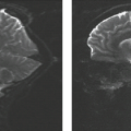
 FIGURE 10.7 Multiple hemorrhagic cavernomas, 1.5 T GRE versus 3 T GRE versus 3 T FSE. Even though some lesions are visible on the 1.5 T GRE image (A), the hypointensity of those lesions is more pronounced on the 3 T GRE (B) and more lesions are demonstrated at 3 T (B). The lesions are either less well seen or invisible on 3 T FSE image (C). |
 FIGURE 10.8 Timing diagrams for spin-echo (A), gradient–recalled echo (B), and echo planar (C) pulse sequences showing the radiofrequency pulses (90, 180, and α degrees) and two in-plane spatial-encoding gradients. (The slice-selection gradient is not shown because it is the same in all sequences.) |
Over the recent years, it has become routine that screening brain MR protocols use faster scanning methods, including sequences like fast spin echo (FSE) rather than conventional spin-echo techniques. This time-saving method has been incorporated into most clinical protocols because of improvements in gradient switching technology, which has permitted shortening of the interecho time τcpmg and an increase in the number of echoes per TR. This sequence differs from the conventional spin-echo sequence by using a train of 180-degree RF pulses to generate a set of echoes that are individually spatially encoded during a single TR. This significantly shortens the total acquisition time because several spatial encoding steps are performed in a single pulse train. The implications in the setting of cerebral hematoma are that dephasing effects in the presence of heterogeneous magnetic susceptibilities are virtually eliminated by the generation of spin echoes. Moreover, the short τcpmg minimizes the signal loss effects of diffusion (Fig. 10.10). Hence, “T2-weighted” FSE has lower sensitivity for the hypointensity of both acute and remote hemorrhages than conventional spin-echo images. If the clinical history suggests that hemorrhage may be present, supplemental GRE or SWI scanning should be used (Figs. 10.7, 10.11, and 10.12).
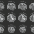
Echo planar imaging (EPI) and other very fast acquisition sequences are now available on virtually all mid- and high-field MR scanners. The main impetus for these “ultrafast” sequences is recent advances in the therapy of acute stroke, the high value of diffusion-weighted imaging, the use of 3D techniques, and a small but increasing demand for the real-time exploration of brain function. These applications require very fast scanning, and many of them are performed with special EPI-capable hardware and software. The EPI sequence uses a single RF pulse train of either spin-echo or GRE format with a complete two-dimensional spatial-encoding scheme of gradient switching (“single-shot EPI”). Various ways of implementing the readout gradients are available and are outside the scope of this chapter (43). The advantage of the EPI method is the very high temporal resolution: images of the brain can be obtained on the order of tens of milliseconds. EPI methods are being used for diffusion-weighted MR, perfusion-weighted MR, and task-activation MR. Generally, EPI methods are very sensitive to magnetic susceptibility effects in both the spin-echo and GRE modes due to the nature of the variable readout gradients (note that in spin-echo EPI, only a single 180-degree RF pulse is used to generate an echo at the selected TE, whereas many gradient reversals are used without 180-degree pulses; i.e., even spin-echo EPI uses gradient refocusing) (Fig. 10.13). It is not only the difference of appearance of hemorrhage on EPI-based sequences that is important. Perhaps most important is the
understanding of when to use EPI-type sequences to assist in either hemorrhage detection or delineation of the etiology of already recognized hemorrhage (see MR Patterns Specific for Clinical Etiologies of Intraparenchymal Hemorrhage).
understanding of when to use EPI-type sequences to assist in either hemorrhage detection or delineation of the etiology of already recognized hemorrhage (see MR Patterns Specific for Clinical Etiologies of Intraparenchymal Hemorrhage).
 FIGURE 10.9 Sensitivity of GRE versus SWI to T2-shortening. 3 T GRE images (A) is normal except for a possible tiny dot of low signal in the right parietal white matter, a lesion clearly demonstrated along with others on 3 T SWI (arrows, B). It is uncertain how many of these low signal “foci” represent tiny hemorrhages or simply ends of veins. Note markedly low signal in normal intramedullary veins traversing brain parenchyma on SWI (B). |
 FIGURE 10.10 Effect of interecho time τcpmg: spin echo versus fast spin echo (FSE). Axial images were obtained with the same repetition time (TR) and echo time (TE) (or effective TE), using conventional spin-echo (A) and FSE (B) sequences in a patient with multiple cavernous hemangiomas. Note that with the use of a long τcpmg in conventional spin echo (A), the acute pineal region hemorrhage is markedly hypointense, whereas with the use of a short τcpmg in FSE (B) the lesion is less hypointense. These differences are seen despite the fact that the same TR and TE are used in these two images. |
 FIGURE 10.11 Acute infarction with hemorrhage. Computed tomography (A) and conventional T2-weighted magnetic resonance (B) clearly demonstrate acute right middle cerebral artery infarction, but only gradient-recalled echo (C) shows markedly hypointense hemorrhage scattered throughout the lesion. |
 FIGURE 10.12 Multiple acute hemorrhages in diffuse axonal injury, fast spin echo (FSE) versus gradient-recalled echo (GRE). T2-weighted FSE images (A) do not reveal any of the numerous hemorrhages clearly seen on the GRE images (B) in the brainstem, corpus callosum, and white matter. |
 FIGURE 10.13 Comparison of fast spin echo (FSE), echo planar imaging (EPI), and gradient-recalled echo (GRE) for acute hemorrhage. Acute hemorrhage within cerebral infarction as marked hypointensity is increasingly more visible and more extensive going from the FSE (left) to the spin echo EPI (middle) to the GRE (right) image. |
Evolution of Intraparenchymal Hematomas
Using the concepts of relaxation discussed in the preceding sections, it is possible to understand the appearance of the various stages in the biochemical evolution of intracranial hemorrhage. The fundamental reason why hemorrhage is unique on MR is that most blood breakdown products are paramagnetic, and they are paramagnetic because of unpaired electrons of their associated iron moiety (Table 10.7). Although some variations can certainly occur, most intracranial hematomas behave in a predictable fashion as they change over time (Table 10.8).
The exact time course of biochemical changes (44) may vary, depending on the pathophysiologic state and on specific imaging technical factors (Tables 10.1 and 10.2). In truth, the clinical dating of the actual hemorrhagic event is notoriously inaccurate, so the nomenclature of the temporal stages of hematomas (i.e., acute, subacute, and chronic) is somewhat arbitrary. Of those factors that are intrinsic to the anatomy and pathophysiology of the lesion, those known to be most important to image interpretation include the age of the hemorrhage, the location of the hematoma (i.e., intraaxial vs. extraaxial, subarachnoid vs. subdural/epidural) (45), and the presence of an underlying lesion (46,47) that affects the blood–brain barrier (47) and the repair response mounted by the patient. Well-vascularized regions, for instance, are expected to show a faster repair response than poorly vascularized regions. Such variability has been reported from biochemical studies of hemorrhage outside of the central nervous system (48). As stated earlier, the radiologist must also be cognizant of the operator-dependent factors that potentially change the MR appearance of hemorrhage (Table 10.2), including the main magnetic field strength, the exact pulse sequence parameters used (37,49), and the method of echo formation (i.e., spin echo, GRE, FSE, or EPI) (6,49). For instance, the signal loss related to the presence of intracellular paramagnetic deoxyhemoglobin and intracellular methemoglobin will be far more evident on 3-T images and seen earlier than on 1.5-T scans. Note that in the following discussion, all T1-weighted images are spin echo unless otherwise stated, and T2-weighted images are generated from conventional spin-echo or FSE techniques. T1-weighted images used TR of 500 to 800 ms and TE of 10 to 25 ms. T2-weighted images used TR of 2,500 to 4,000 ms, and TEs (or effective TEs) were long (greater than 70 ms).
TABLE 10.7 Unpaired Electrons Associated with Blood-Breakdown Products | ||||||||||||||||||
|---|---|---|---|---|---|---|---|---|---|---|---|---|---|---|---|---|---|---|
|
It has become generally accepted that evolving intracranial hematomas typically change over time mainly, but not exclusively, in two important ways that alter MR signal intensity patterns: the oxygenation state of hemoglobin changes, and initially intact RBC membranes eventually lyse (Fig. 10.14). As the oxygenation state of the hemoglobin molecule changes with hematoma evolution, it is the iron moiety associated with hemoglobin that most directly influences changes in MR signal intensity. The magnetic properties of iron, determined by its electronic configuration, vary with its biochemical form, spatial distribution, and oxidation state. The changing electronic configuration is summarized in Table 10.9 to demonstrate how the magnetic properties of hemorrhage and hence the nuclear relaxation processes that underlie the signal contrast in the MR image depend on the biochemical pathways of iron metabolism.
Although iron is the most abundant transition metal in the human body, being vital for oxygen transport by hemoglobin in the erythrocyte of blood and many catalytic processes involving enzymes, free iron is toxic, as is demonstrated by toxic ingestions and iron overload states (50,51,52). The toxicity, believed to be due to enhanced free radical production by unchelated iron (53), requires that all iron be tightly bound in well-controlled metabolic pathways of absorption, transport, storage, and conversion into functional end products. The repair of hemorrhage requires a tightly controlled iron salvage pathway in which iron from the extravasated erythrocytes is mobilized from hemoglobin, detoxified by chelation to short-term iron transport proteins for transfer back to the reticuloendothelial system, or converted to long-term storage proteins for local deposition (51,54,55).
TABLE 10.8 General Guidelines for Temporal Evolution of Intracranial Hematomas at 1.5 T | |||||||||||||||||||||||||||||||||||
|---|---|---|---|---|---|---|---|---|---|---|---|---|---|---|---|---|---|---|---|---|---|---|---|---|---|---|---|---|---|---|---|---|---|---|---|
| |||||||||||||||||||||||||||||||||||
Related posts:
Stay updated, free articles. Join our Telegram channel

Full access? Get Clinical Tree


