Fig. 1
Invariant shape similarity
Problems
Since nonrigid shapes are ubiquitous in the world and are encountered at all scales from macro to nano, nonrigid shape similarity plays a key role in many applications in imaging sciences, pattern recognition, computer vision, and computer graphics. Two archetype problems in shape analysis considered in this chapter are invariant similarity and correspondence. As will be discussed in the following, these two problems are interrelated: finding the best correspondence between two shapes also allows quantifying their similarity.
A good example of shape similarity is the problem of face recognition [19, 21, 24]. As the crudest approximation, one can think of faces as rigid surfaces and compare them using similarity criteria invariant under rigid transformations. However, such an approach does not account for surface deformations due to facial expressions, which can be approximated by inelastic deformations. Accounting for such deformations requires different similarity criteria. Yet, even elastic deformations are not enough to model the behavior of human faces: many facial expresses involve elastic deformations that change the facial shape topology (think of open and closed mouth). This extension of the model will require revisiting the similarity criterion once again.
The problem of correspondence is often encountered in shape synthesis applications such as morphing. In order to morph one shape into the other, one needs to know which point on the first shape will be transformed into a point on the second shape, in other words, establishing a correspondence between the shapes.
Methods
Many different approaches to shape similarity and correspondence can be considered as instances of the minimum-distortion correspondence problem, in which two shapes are endowed with certain structure, and one attempts to find the best (least distorting) matching between these structures. Such structures can be local (e.g., multiscale heat kernel signatures [106], local photometric properties [107, 119], or conformal factor [12]) or global (e.g., geodesic [24, 47, 78], diffusion [28], and commute time [31]) distances. The distortion of the best possible correspondence can be used as a criterion of shape similarity. By defining a structure invariant under certain class of transformations, it is possible to obtain invariant correspondence or similarity.
Local structures can be regarded as feature descriptors. As a model for global structures, metric spaces are used.
Chapter Outline
This chapter tries to present a unifying view on the archetypical problems in shape analysis. The first part presents a metric view on the problem of nonrigid shape similarity and correspondence, a common denominator allowing to deal with different types of invariance. According to this model, shapes are represented as metric spaces. The mathematical foundations of this model are provided in Sect. 2. Sections 3 and 4 deal with discrete representation of shapes, which is of essence in practical numerical computations. Section 5 provides a rigorous formulation of the invariant shape similarity problem and reviews different algorithms for its computation. Section 6 deals with an extension of invariant similarity to shapes which are partially similar, and Sect. 7 deals with a particular case of self-similarity and symmetry. Local feature-based methods and their use to create global shape descriptors are presented in Sect. 8. Finally, concluding remarks in Sect. 9 end the chapter. This chapter is based in part on the book [26], to which the reader is referred for further discussion and details.
2 Shapes as Metric Spaces
Elad and Kimmel [47, 48], Mémoli and Sapiro [78], and Bronstein et al. [23, 24] suggested to model shapes as metric spaces. The key idea of this model is that it allows to compare shapes as metric spaces. Since the model allows arbitrarity in the definition of the metric, desired invariance considerations guide the choice of the metric.
This section introduces the mathematical formalism and notation of this model and shows the construction of three different types of metric geometries: Euclidean, Riemannian, and diffusion.
Basic Notions
Topological Spaces
Given a set X, a topology T on X is a collection of subsets of X satisfying (Ti) X, 0 ∈ T; (Tii)  for U α ∈ T; and (Tiii)
  for U i ∈ T. X together with T is called a topological space. By convention, sets in T are referred to as open sets and their complements as closed sets.
for U α ∈ T; and (Tiii) for U i ∈ T. X together with T is called a topological space. By convention, sets in T are referred to as open sets and their complements as closed sets. A neighborhood N(x) of x is a set containing an open set U ∈ T such that x ∈ U. Points with neighborhood are called interior.
A topological space is called Hausdorff if distinct points in it have disjoint neighborhoods.
Two topological spaces X and Y are homeomorphic if there exists bijection  which is continuous and has continuous inverse α −1. Since homeomorphisms copy topologies, homeomorphic spaces are topologically equivalent [1].
which is continuous and has continuous inverse α −1. Since homeomorphisms copy topologies, homeomorphic spaces are topologically equivalent [1].Metric Spaces
A function  which is (Mi) positive-definite (d(x, y) > 0 for all x ≠ y and d(x, y) = 0 for x = y) and (Mii) subadditive (d(x, z) ≤ d(x, y) + d(y, z) for all x, y, z) is called a metric on X. The metric is an abstraction of the notion of distance between pairs of points on X. Property (Mii) is called triangle inequality and generalizes the known fact: the sum of the lengths of two edges of a triangle is greater or equal to the length of the third edge. The pair (X, d) is called a metric space.
which is (Mi) positive-definite (d(x, y) > 0 for all x ≠ y and d(x, y) = 0 for x = y) and (Mii) subadditive (d(x, z) ≤ d(x, y) + d(y, z) for all x, y, z) is called a metric on X. The metric is an abstraction of the notion of distance between pairs of points on X. Property (Mii) is called triangle inequality and generalizes the known fact: the sum of the lengths of two edges of a triangle is greater or equal to the length of the third edge. The pair (X, d) is called a metric space. A metric induces topology through the definition of open metric ball B r (x) = { x ′ ∈ X: d(x, x ′ ) < r}. A neighborhood of x in a metric space is a set containing a metric ball B r (x) [34].
Isometries
Given two metric spaces (X, d) and (Y, δ), the set  of pairs such that for every x ∈ X there exists at least one y ∈ Y such that (x, y) ∈ C, and similarly, for every y ∈ Y, there exists an x ∈ X such that (x, y) ∈ C is called a correspondence between X and Y. Note that a correspondence C is not necessarily a function. The correspondence is called bijective if every point in X has a unique corresponding point in Y and vice versa.
of pairs such that for every x ∈ X there exists at least one y ∈ Y such that (x, y) ∈ C, and similarly, for every y ∈ Y, there exists an x ∈ X such that (x, y) ∈ C is called a correspondence between X and Y. Note that a correspondence C is not necessarily a function. The correspondence is called bijective if every point in X has a unique corresponding point in Y and vice versa.The discrepancy of the metrics d and δ between the corresponding points is called the distortion of the correspondence,
Metric spaces (X, d) and (Y, δ) are said to be ε–isometric if there exists a correspondence C with dis(C) ≤ ε. Such a C is called an ε–isometry.
A particular case of a 0-isometry is called an isometry. In this case, the correspondence is a bijection and X and Y are called isometric.
Euclidean Geometry
Euclidean space  (hereinafter also denoted as
  ) with the Euclidean metric
  is the simplest example of a metric space. Given as a subset X of
  , we can measure the distances between points x and x ′ on X using the restricted Euclidean metric,
 for all x, x ′ in X.
(hereinafter also denoted as ) with the Euclidean metric is the simplest example of a metric space. Given as a subset X of , we can measure the distances between points x and x ′ on X using the restricted Euclidean metric,The restricted Euclidean metric  is invariant under Euclidean transformations of X, which include translation, rotation, and reflection in
  . In other words, X and its Euclidean transformation i(X) are isometric in the sense of the Euclidean metric. Euclidean isometries are called congruences, and two subsets of
  differing up to a Euclidean isometry are said to be congruent.
is invariant under Euclidean transformations of X, which include translation, rotation, and reflection in . In other words, X and its Euclidean transformation i(X) are isometric in the sense of the Euclidean metric. Euclidean isometries are called congruences, and two subsets of differing up to a Euclidean isometry are said to be congruent.Riemannian Geometry
Manifolds
A Hausdorff space X which is locally homeomorphic to  (i.e., for every x in X, there exists a neighborhood U and a homeomorphism
  ) is called an n–manifold or an n–dimensional manifold. The function α is called a chart. A collection of neighborhoods that cover X together with their charts is called an atlas on X. Given two charts α and β with overlapping domains U and V, the map
  is called a transition function. A manifold whose transition functions are all differentiable is called a differentiable manifold. More generally a
  –manifold has all transition maps k-times continuously differentiable. A
  -manifold is called smooth.
(i.e., for every x in X, there exists a neighborhood U and a homeomorphism ) is called an n–manifold or an n–dimensional manifold. The function α is called a chart. A collection of neighborhoods that cover X together with their charts is called an atlas on X. Given two charts α and β with overlapping domains U and V, the map is called a transition function. A manifold whose transition functions are all differentiable is called a differentiable manifold. More generally a –manifold has all transition maps k-times continuously differentiable. A -manifold is called smooth. A manifold with boundary is not a manifold in the strict sense of the above definition. Its interior points are locally homeomorphic to  , and every point on the boundary ∂ X is homeomorphic to
  .
.
, and every point on the boundary ∂ X is homeomorphic to .Of particular interest for the discussion in this chapter are two-dimensional (n = 2) manifolds, which model boundaries of physical objects in the world surrounding us. Such manifolds are also called surfaces. In the following, when referring to shapes and objects, the terms manifold, surface, and shape will be used synonymously.
Differential Structures
Locally, a manifold can be represented as a linear space, in the following way. Let  be a chart on a neighborhood of x and
  be a differentiable curve passing through x = γ(0). The derivative of the curve
  is called a tangent vector at x. The set of all equivalence classes of tangent vectors at x forming an n-dimensional real vector space is called the tangent space T x X at x.
be a chart on a neighborhood of x and be a differentiable curve passing through x = γ(0). The derivative of the curve is called a tangent vector at x. The set of all equivalence classes of tangent vectors at x forming an n-dimensional real vector space is called the tangent space T x X at x. A family of inner products  depending smoothly on x is called Riemannian metric tensor. A manifold X with a Riemannian metric tensor is called a Riemannian manifold.
depending smoothly on x is called Riemannian metric tensor. A manifold X with a Riemannian metric tensor is called a Riemannian manifold. The Riemannian metric allows to define local length structures and differential calculus on the manifold. Given a differentiable scalar-valued function  , the exterior derivative (differential) is a form
  on the tangent space TX. For a tangent vector
  ,
,  . ∇f is called the gradient of f at x and is a natural generalization of the notion of the gradient in vector spaces to manifolds. Similarly to the definition of Laplacian satisfying
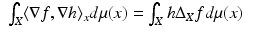 for differentiable scalar-valued functions f and h, the operator
  is called the Laplace–Beltrami operator, a generalization of the Laplacian. Here, μ denotes the measure associated with the n-dimensional volume element (area element for n = 2). The Laplace–Beltrami operator is (Li) symmetric (
 ), (Lii) of local action (
 is independent of the value of f(x ′ ) for x ′ ≠ x), and (Liii) positive semi-definite (
 ) (in many references, the Laplace–Beltrami is defined as a negative semi-definite operator) and (Liv) coincides with the Laplacian on Euclidean domains, such that
  if f is a linear function and X is Euclidean.
, the exterior derivative (differential) is a form on the tangent space TX. For a tangent vector , . ∇f is called the gradient of f at x and is a natural generalization of the notion of the gradient in vector spaces to manifolds. Similarly to the definition of Laplacian satisfying is called the Laplace–Beltrami operator, a generalization of the Laplacian. Here, μ denotes the measure associated with the n-dimensional volume element (area element for n = 2). The Laplace–Beltrami operator is (Li) symmetric (), (Lii) of local action ( is independent of the value of f(x ′ ) for x ′ ≠ x), and (Liii) positive semi-definite () (in many references, the Laplace–Beltrami is defined as a negative semi-definite operator) and (Liv) coincides with the Laplacian on Euclidean domains, such that if f is a linear function and X is Euclidean. Geodesics
Another important use of the Riemannian metric tensor is to measure the length of paths on the manifold. Given a continuously differentiable curve ![$$\gamma: [a,b] \rightarrow X$$](/wp-content/uploads/2016/04/A183156_2_En_57_Chapter_IEq33.gif) , its length is given by
, its length is given by
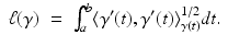 For the set of all continuously differentiable curves
  between the points x, x ′ ,
defines a metric on X referred to as length or geodesic metric. If the manifold is compact, for any pair of points x and x ′ , there exists a curve  called a minimum geodesic such that
 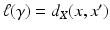 .
.
, its length is given by between the points x, x ′ ,(1)
called a minimum geodesic such that . Embedded Manifolds
A particular realization of a Riemannian manifold called embedded manifold (or embedded surface for n = 2) is a smooth submanifold of  (m > n). In this case, the tangent space is an n-dimensional hyperplane in
  , and the Riemannian metric is defined as the restriction of the Euclidean inner product to the tangent space,
  .
.
(m > n). In this case, the tangent space is an n-dimensional hyperplane in , and the Riemannian metric is defined as the restriction of the Euclidean inner product to the tangent space, .The length of a curve ![$$\gamma: [a,b] \rightarrow X \subset \mathbb{R}^{m}$$](/wp-content/uploads/2016/04/A183156_2_En_57_Chapter_IEq40.gif) on an embedded manifold is expressed through the Euclidean metric,
on an embedded manifold is expressed through the Euclidean metric,
and the geodesic metric d X defined according to (1) is said to be induced by  . (Repeating the process, one obtains that the metric induced by d X is equal to d X . For this reason, d X is referred to as intrinsic metric [34].)
on an embedded manifold is expressed through the Euclidean metric,(2)
. (Repeating the process, one obtains that the metric induced by d X is equal to d X . For this reason, d X is referred to as intrinsic metric [34].) Though apparently embedded manifolds are a particular case of a more general notion of Riemannian manifolds, it appears that any Riemannian manifold can be realized as an embedded manifold. This is a consequence of the Nash embedding theorem [84], showing that a  Riemannian manifold can be isometrically embedded in a Euclidean space of dimension m = n 2 + 5n + 3. In other words, any smooth Riemannian manifold can be defined as a metric space which is isometric to a smooth submanifold of a Euclidean space with the induced metric.
Riemannian manifold can be isometrically embedded in a Euclidean space of dimension m = n 2 + 5n + 3. In other words, any smooth Riemannian manifold can be defined as a metric space which is isometric to a smooth submanifold of a Euclidean space with the induced metric.Rigidity
Riemannian manifolds do not have a unique realization as embedded manifolds. One obvious degree of freedom is the set of all Euclidean isometries: two congruent embedded manifolds are isometric and thus are realizations of the same Riemannian manifold. However, a Riemannian manifold may have two realizations which are isometric but incongruent. Such manifolds are called nonrigid. If, on the other hand, a manifold’s only isometries are congruences, it is called rigid.
Diffusion Geometry
Another type of metric geometry arises from the analysis of heat propagation on manifolds. This geometry is called diffusion and is also intrinsic. We start by reviewing properties of diffusion operators.
Diffusion Operators
A function  is called a diffusion kernel if it satisfies the following properties: (Ki) nonnegativity: k(x, x) ≥ 0; (Kii) symmetry: k(x, y) = k(y, x); (Kiii) positive-semidefiniteness: for every bounded f,
 (Kiv) square integrability:
  ; and (Kv) conservation:
  (y) = 1. The value of k(x, y) can be interpreted as a transition probability from x to y by one step of a random walk on X.
is called a diffusion kernel if it satisfies the following properties: (Ki) nonnegativity: k(x, x) ≥ 0; (Kii) symmetry: k(x, y) = k(y, x); (Kiii) positive-semidefiniteness: for every bounded f,; and (Kv) conservation: (y) = 1. The value of k(x, y) can be interpreted as a transition probability from x to y by one step of a random walk on X.Diffusion kernel defines a linear operator
which is known to be self-adjoint. Because of (Kiv),  has a finite Hilbert norm and therefore is compact. As the result, it admits a discrete eigendecomposition
  with some eigenfunctions
  and eigenvalues
  . α i ≥ 0 by virtue of property (Kiii), and α i ≤ 1 by virtue of (Kv) and consequence of the Perron–Frobenis theorem.
(3)
has a finite Hilbert norm and therefore is compact. As the result, it admits a discrete eigendecomposition with some eigenfunctions and eigenvalues . α i ≥ 0 by virtue of property (Kiii), and α i ≤ 1 by virtue of (Kv) and consequence of the Perron–Frobenis theorem.By the spectral theorem, the diffusion kernel can be presented as  . Since
  form an orthonormal basis of L 2(X),
a fact sometimes referred to as Parseval’s theorem. Using these results, properties (Kiii–Kv) can be rewritten in the spectral form as 0 ≤ α i ≤ 1 and  .
.
. Since form an orthonormal basis of L 2(X),(4)
.An important property of diffusion operators is the fact that for every t ≥ 0, the operator  is also a diffusion operator with the eigenbasis of
  and corresponding eigenvalues
  . The kernel of
  expresses the transition probability by random walk of t steps. This allows to define a scale space of kernels,
  , with the scale parameter t.
is also a diffusion operator with the eigenbasis of and corresponding eigenvalues . The kernel of expresses the transition probability by random walk of t steps. This allows to define a scale space of kernels, , with the scale parameter t.There exist a large variety of possibilities to define a diffusion kernel and the related diffusion operator. Here, we restrict our attention to operators describing heat diffusion. Heat diffusion on surfaces is governed by the heat equation
where u(x, t) is the distribution of heat on the surface at point x in time t, u 0 is the initial heat distribution, and  is the positive-semidefinite Laplace–Beltrami operator, a generalization of the second-order Laplacian differential operator
  to non-Euclidean domains. (If X has a boundary, boundary conditions should be added.)
(5)
is the positive-semidefinite Laplace–Beltrami operator, a generalization of the second-order Laplacian differential operator to non-Euclidean domains. (If X has a boundary, boundary conditions should be added.)On Euclidean domains ( ), the classical approach to the solution of the heat equation is by representing the solution as a product of temporal and spatial components. The spatial component is expressed in the Fourier domain, based on the observation that the Fourier basis is the eigenbasis of the Laplacian
  , and the corresponding eigenvalues are the frequencies of the Fourier harmonics. A particular solution for a point initial heat distribution u 0(x) = δ(x − y) is called the heat kernel
  , which is shift invariant in the Euclidean case. A general solution for any initial condition u 0 is given by convolution
  , where
  is referred to as heat operator.
), the classical approach to the solution of the heat equation is by representing the solution as a product of temporal and spatial components. The spatial component is expressed in the Fourier domain, based on the observation that the Fourier basis is the eigenbasis of the Laplacian , and the corresponding eigenvalues are the frequencies of the Fourier harmonics. A particular solution for a point initial heat distribution u 0(x) = δ(x − y) is called the heat kernel , which is shift invariant in the Euclidean case. A general solution for any initial condition u 0 is given by convolution , where is referred to as heat operator. In the non-Euclidean case, the eigenfunctions of the Laplace–Beltrami operator  can be regarded as a “Fourier basis” and the eigenvalues given the “frequency” interpretation. The heat kernel is not shift invariant but can be expressed as
  .
.
can be regarded as a “Fourier basis” and the eigenvalues given the “frequency” interpretation. The heat kernel is not shift invariant but can be expressed as .It can be shown that the heat operator is related to the Laplace–Beltrami operator as  , and as a result, it has the same eigenfunctions ϕ i and corresponding eigenvalues
  . It can be thus seen as a particular instance of a more general family of diffusion operators
  diagonalized by the eigenbasis of the Laplace–Beltrami operator, namely,
  ’s as defined in the previous section but restricted to have the eigenfunctions ψ i = ϕ i . The corresponding diffusion kernels can be expressed as
where K(λ) is some function such that α i = K(λ i ) (in the case of  , K(λ) = e −t λ ). Since the Laplace–Beltrami eigenvalues can be interpreted as frequency, K(λ) can be thought of as the transfer function of a low-pass filter. Using this signal processing analogy, the kernel k(x, y) can be interpreted as the point spread function at a point y, and the action of the diffusion operator
  on a function f on X can be thought of as the application of the point spread function by means of a non shift-invariant version of convolution. The transfer function of the diffusion operator
  is K t (λ), which can be interpreted as multiple applications of the filter K(λ). Such multiple applications decrease the effective bandwidth of the filter and, consequently, increase its effective support in space. Because of this duality, both k(x, y) and K(λ) are often referred to as diffusion kernels.
, and as a result, it has the same eigenfunctions ϕ i and corresponding eigenvalues . It can be thus seen as a particular instance of a more general family of diffusion operators diagonalized by the eigenbasis of the Laplace–Beltrami operator, namely, ’s as defined in the previous section but restricted to have the eigenfunctions ψ i = ϕ i . The corresponding diffusion kernels can be expressed as(6)
, K(λ) = e −t λ ). Since the Laplace–Beltrami eigenvalues can be interpreted as frequency, K(λ) can be thought of as the transfer function of a low-pass filter. Using this signal processing analogy, the kernel k(x, y) can be interpreted as the point spread function at a point y, and the action of the diffusion operator on a function f on X can be thought of as the application of the point spread function by means of a non shift-invariant version of convolution. The transfer function of the diffusion operator is K t (λ), which can be interpreted as multiple applications of the filter K(λ). Such multiple applications decrease the effective bandwidth of the filter and, consequently, increase its effective support in space. Because of this duality, both k(x, y) and K(λ) are often referred to as diffusion kernels.Diffusion Distances
Since a diffusion kernel k(x, y) measures the degree of proximity between x and y, it can be used to define a metric
on X, which was first constructed by Berard et al. in [*] and dubbed as the diffusion distance by Coifman and Lafon [40]. Another way to interpret the latter distance is by considering the embedding 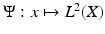 by which each point x on X is mapped to the function
  . The embedding
  is an isometry between X equipped with diffusion distance and L 2(X) equipped with the standard L 2 metric, since
 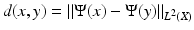 . Because of spectral duality, the diffusion distance can also be written as
Here as well we can define an isometric embedding  with
with 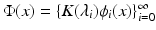 , termed as the diffusion map by Lafon. The diffusion distance can be cast as
 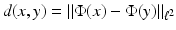 .
.
(7)
by which each point x on X is mapped to the function . The embedding is an isometry between X equipped with diffusion distance and L 2(X) equipped with the standard L 2 metric, since . Because of spectral duality, the diffusion distance can also be written as(8)
with , termed as the diffusion map by Lafon. The diffusion distance can be cast as . The same way a diffusion operator  defines a scale space, a family of diffusion metrics can be defined for t ≥ 0 as
where 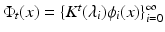 . Interpreting diffusion processes as random walks, d t can be related to the “connectivity” of points x and y by walks of length t (the more such walks exist, the smaller is the distance).
defines a scale space, a family of diffusion metrics can be defined for t ≥ 0 as(9)
. Interpreting diffusion processes as random walks, d t can be related to the “connectivity” of points x and y by walks of length t (the more such walks exist, the smaller is the distance).The described framework is very generic, leading to numerous potentially useful diffusion geometries parametrized by the selection of the transfer function K(λ). Two particular choices are frequent in shape analysis, the first one being the heat kernel, K t (λ) = e −t λ , and the second one being the commute time kernel,  , resulting in the heat diffusion and commute time metrics, respectively. While the former kernel involves a scale parameter, typically tuned by hand, the latter one is scale invariant, meaning that neither the kernel nor the diffusion metric it induces changes under uniform scaling of the embedding coordinates of the shape.
, resulting in the heat diffusion and commute time metrics, respectively. While the former kernel involves a scale parameter, typically tuned by hand, the latter one is scale invariant, meaning that neither the kernel nor the diffusion metric it induces changes under uniform scaling of the embedding coordinates of the shape.3 Shape Discretization
In order to allow storage and processing of a shape by a digital computer, it has to be discretized. This section reviews different notions in the discrete representation of shapes.
Sampling
Sampling is the reduction of the continuous surface X representing a shape into a finite discrete set of representative points 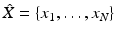 . The number of points
  is called the size of the sampling. The radius of the sampling refers to the smallest positive scalar r for which
  is an r-covering of X, i.e.,
The sampling is called s-separated if d X (x i , x j ) ≥ s for every distinct  .
.
. The number of points is called the size of the sampling. The radius of the sampling refers to the smallest positive scalar r for which is an r-covering of X, i.e.,(10)
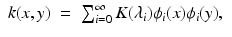
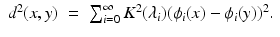
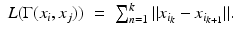
.Sampling partitions the continuous surface into a set of disjoint regions,
called the Voronoi regions [7] (Fig. 2). A Voronoi region V i contains all the points on X that are closer to x i than to any other x j . That the sampling is said to induce a Voronoi tessellation (Unlike in the Euclidean case where every sampling induces a valid tessellation (cell complex), samplings of curved surfaces may result in Voronoi regions that are not valid cells, i.e., are not homeomorphic to a disk. In [66], Leibon and Letscher showed that an r-separated sampling of radius r with r smaller than  of the convexity radius of the shape is guaranteed to induce a valid tessellation.) which we denote by
  .
.
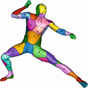
(11)
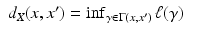
of the convexity radius of the shape is guaranteed to induce a valid tessellation.) which we denote by .Fig. 2
Voronoi decomposition of a surface with a non-Euclidean metric
Sampling can be regarded as a quantization process in which a point x on the continuous surface is represented by the closest x i in the sampling [51]. Such a process can be expressed as a function mapping each V i to the corresponding (Points on the boundary of the Voronoi regions are equidistant from at least two sample points and therefore can be mapped arbitrarily to any of them.) sample x i . Intuitively, the smaller are the Voronoi regions, the better is the sampling. Sampling quality is quantified using an error function. For example,

determines the maximum size of the Voronoi regions. If the shape is further equipped with a measure (e.g., the standard area measure), other error functions can be defined, e.g.,
In what follows, we will show sampling procedures optimal or nearly optimal in terms of these criteria.
(12)
(13)
Farthest Point Sampling
Farthest point sampling (FPS) is a greedy procedure constructing a sequence of samplings  . A sampling
  is constructed from
  by adding the farthest point

The sequence {r N } of the sampling radii associated with  is nonincreasing, and, furthermore, each
  is also r N -separated. The starting point x 1 is usually picked up at random, and the stopping condition can be either the sampling size or radius.
. A sampling is constructed from by adding the farthest point(14)
is nonincreasing, and, furthermore, each is also r N -separated. The starting point x 1 is usually picked up at random, and the stopping condition can be either the sampling size or radius.Though FPS does not strictly minimize any of the error criteria defined in the previous section, in terms of ε ∞ , it is no more than twice inferior to the optimal sampling of the same size [59]. In other words, for  produced using FPS,
This result is remarkable, as finding the optimal sampling is known to be an NP-hard problem.
produced using FPS,(15)
Centroidal Voronoi Sampling
In order for a sampling to be ε 2-optimal, each sample x i has to minimize
A point minimizing the latter quantity is referred to as the centroid of V i . Therefore, an ε 2-optimal sampling induces a so-called centroidal Voronoi tessellation (CVT), in which the centroid of each Voronoi region coincides with the sample point inducing it [45, 90]. Such a tessellation and the corresponding centroidal Voronoi sampling are generally not unique.
(16)
A numerical procedure for the computation of a CVT of a shape is known as the Lloyd–Max algorithm [68, 73]. Given some initial sampling  of size N (produced, e.g., using FPS), the Voronoi tessellation induced by it is computed. The centroids of each Voronoi region are computed, yielding a new sampling
  of size N. The process is repeated iteratively until the change of
  becomes insignificant. While producing high-quality samplings in practice, the Lloyd–Max procedure is guaranteed to converge only to a local minimum of ε 2. For computational aspects of CVTs on meshes, the reader is referred to [90].
of size N (produced, e.g., using FPS), the Voronoi tessellation induced by it is computed. The centroids of each Voronoi region are computed, yielding a new sampling of size N. The process is repeated iteratively until the change of becomes insignificant. While producing high-quality samplings in practice, the Lloyd–Max procedure is guaranteed to converge only to a local minimum of ε 2. For computational aspects of CVTs on meshes, the reader is referred to [90].Shape Representation
Once the shape is sampled, it has to be represented in a way allowing computation of discrete geometric quantities associate with it.
Simplicial Complexes
The simplest representation of a shape is obtained by considering the points of the sampling as points in the ambient Euclidean space. Such a representation is usually referred to as a point cloud. Points in the cloud are called vertices and denoted by  . The notion of a point cloud can be generalized using the formalism of simplical complexes. For our purpose, an abstract k–simplex is a set of cardinality k + 1. A subset of a simplex is called a face. A set K of simplices is said to be an abstract simplical complex if any face of σ ∈ K is also in K, and the intersection of any two simplices σ 1, σ 2 ∈ K is a face of both σ 1 and σ 2. A simplicial k-complex is a simplicial complex in which the largest dimension of any simplex is k. A simplicial k-complex is said to be homogeneous if every simplex of dimension less than k is the face of some k-simplex. A topological realization
  of a simplicial complex K maps K to a simplicial complex in
  , in which vertices are identified with the canonical basis of
  , and each simplex in K is represented as the convex hull of the corresponding points
  . A geometric realization
  is a map of the simplicial complex
  to
to  defined by associating the standard basis vectors
  with the vertex positions
  .
.
. The notion of a point cloud can be generalized using the formalism of simplical complexes. For our purpose, an abstract k–simplex is a set of cardinality k + 1. A subset of a simplex is called a face. A set K of simplices is said to be an abstract simplical complex if any face of σ ∈ K is also in K, and the intersection of any two simplices σ 1, σ 2 ∈ K is a face of both σ 1 and σ 2. A simplicial k-complex is a simplicial complex in which the largest dimension of any simplex is k. A simplicial k-complex is said to be homogeneous if every simplex of dimension less than k is the face of some k-simplex. A topological realization of a simplicial complex K maps K to a simplicial complex in , in which vertices are identified with the canonical basis of , and each simplex in K is represented as the convex hull of the corresponding points . A geometric realization is a map of the simplicial complex to defined by associating the standard basis vectors with the vertex positions .In this terminology, a point cloud is a simplicial 0-complex having a discrete topology. Introducing the notion of neighborhood, we can define a subset  of pairs of vertices that are adjacent. Pairs of adjacent vertices are called edges, and the simplicial 1-complex
  has a graph topology, i.e., the set of vertices
  forms an undirected graph with the set of edges E. A simplicial 2-complex consisting of vertices, edges, and triangular faces built upon triples of vertices and edges is called a triangular mesh. The mesh is called topologically valid if it is homeomorphic to the underlying continuous surface X. This usually implies that the mesh has to be a two manifold. A mesh is called geometrically valid if it does not contain self-intersecting triangles, which happens if and only if the geometric realization
  of the mesh is bijective. Consequently, any point x on a geometrically valid mesh can be uniquely represented as
  . The vector
  is called the barycentric coordinates of x and has at most three nonzero elements. If the point coincides with a vertex,
  is a canonical basis vector; if the point lies on an edge,
  has two nonzero elements; otherwise,
  has three nonzero elements and x lies on a triangular face.
of pairs of vertices that are adjacent. Pairs of adjacent vertices are called edges, and the simplicial 1-complex has a graph topology, i.e., the set of vertices forms an undirected graph with the set of edges E. A simplicial 2-complex consisting of vertices, edges, and triangular faces built upon triples of vertices and edges is called a triangular mesh. The mesh is called topologically valid if it is homeomorphic to the underlying continuous surface X. This usually implies that the mesh has to be a two manifold. A mesh is called geometrically valid if it does not contain self-intersecting triangles, which happens if and only if the geometric realization of the mesh is bijective. Consequently, any point x on a geometrically valid mesh can be uniquely represented as . The vector is called the barycentric coordinates of x and has at most three nonzero elements. If the point coincides with a vertex, is a canonical basis vector; if the point lies on an edge, has two nonzero elements; otherwise, has three nonzero elements and x lies on a triangular face.A particular way of constructing a triangular mesh stems from the Voronoi tessellation induced by the sampling. We define the simplicial 3-complex as

in which a pair of vertices spans an edge and a triple of vertices spans a face if the corresponding Voronoi regions are adjacent. A mesh defined in this way is called a Delaunay mesh. (Unlike in the Euclidean case where every sampling induces a valid Delaunay triangulation, an invalid Voronoi tessellation results in a topologically invalid Delaunay mesh. In [66], Leibon and Letscher showed that under the same conditions sufficient for the existence of a valid Voronoi tessellation, the Delaunay mesh is also topologically valid.)
(17)
Parametric Surfaces
Shapes homeomorphic to a disk can be parametrized using a single global chart, e.g., on the unit square, ![$${\mathrm{x}}: [0,1]^{2} \rightarrow \mathbb{R}^{3}$$](/wp-content/uploads/2016/04/A183156_2_En_57_Chapter_IEq118.gif) . (Manifolds with more complex topology can still be parametrized in this way by introducing cuts that open the shape into a topological disk.) Such surfaces are called parametric and can be sampled directly in the parametrization domain. For example, if the parametrization domain is sampled on a regular Cartesian grid, the shape can be represented as three N × N arrays of x, y, and z values. Such a completely regular structure is called a geometry image [56, 69, 99] and can be thought indeed as a three-channel image that can undergo standard image processing such as compression. Geometry images are ideally suitable for processing by vector and parallel hardware.
. (Manifolds with more complex topology can still be parametrized in this way by introducing cuts that open the shape into a topological disk.) Such surfaces are called parametric and can be sampled directly in the parametrization domain. For example, if the parametrization domain is sampled on a regular Cartesian grid, the shape can be represented as three N × N arrays of x, y, and z values. Such a completely regular structure is called a geometry image [56, 69, 99] and can be thought indeed as a three-channel image that can undergo standard image processing such as compression. Geometry images are ideally suitable for processing by vector and parallel hardware.
. (Manifolds with more complex topology can still be parametrized in this way by introducing cuts that open the shape into a topological disk.) Such surfaces are called parametric and can be sampled directly in the parametrization domain. For example, if the parametrization domain is sampled on a regular Cartesian grid, the shape can be represented as three N × N arrays of x, y, and z values. Such a completely regular structure is called a geometry image [56, 69, 99] and can be thought indeed as a three-channel image that can undergo standard image processing such as compression. Geometry images are ideally suitable for processing by vector and parallel hardware.Implicit Surfaces
Another way of representing a shape is by considering the isosurfaces  of some function
  defined on a region of
  . Such a representation is called implicit, and it often arises in medical imaging applications, where shapes are two-dimensional boundaries created by discontinuities in volumetric data. Implicit representation can be naturally processed using level-set-based algorithms, and it easily handles arbitrary topology. A disadvantage is the bigger amount of storage commonly required for such representations.
of some function defined on a region of . Such a representation is called implicit, and it often arises in medical imaging applications, where shapes are two-dimensional boundaries created by discontinuities in volumetric data. Implicit representation can be naturally processed using level-set-based algorithms, and it easily handles arbitrary topology. A disadvantage is the bigger amount of storage commonly required for such representations. 4 Metric Discretization
Next step in the discrete representation of shapes is the discretization of the metric.
Shortest Paths on Graphs
The most straightforward approach to metric discretization arises from considering the shape as a graph in which neighbor vertices are connected. A path in the graph between vertices x i , x j is an ordered set of connected edges
where  and
and  . The length of path
  is the sum of its constituent edge lengths,
A minimum geodesic in a graph is the shortest path between the vertices,
We can use 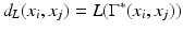 as a discrete approximation to the geodesic metric d X (x i , x j ).
(18)
and . The length of path is the sum of its constituent edge lengths,(19)
(20)
as a discrete approximation to the geodesic metric d X (x i , x j ).According to the Bellman optimality principle [10], given  a shortest path between x i and x j and x k a point on the path, the sub-paths
  and
and  are the shortest paths between x i , x k and x k , x j , respectively. The length of the shortest path in the graph can be thus expressed by the following recursive equation:
a shortest path between x i and x j and x k a point on the path, the sub-paths and are the shortest paths between x i , x k and x k , x j , respectively. The length of the shortest path in the graph can be thus expressed by the following recursive equation:(21)
Dijkstra’s Algorithm
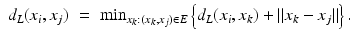
A famous algorithm for the solution of the recursion (21) was proposed by Dijkstra. Dijkstra’s algorithm measures the distance map  from the source vertex x i to all the vertices in the graph.
from the source vertex x i to all the vertices in the graph.Every vertex in Dijkstra’s algorithm is processed exactly once; hence, Nn outer iterations are performed. Extraction of vertex with smallest d is straightforward with  complexity and can be reduced to
  using efficient data structures such as Fibonacci heap. In the inner loop, updating adjacent vertices in our case, since the graph is sparsely connected, is
  . The resulting overall complexity is
  .
.
complexity and can be reduced to using efficient data structures such as Fibonacci heap. In the inner loop, updating adjacent vertices in our case, since the graph is sparsely connected, is . The resulting overall complexity is . Metrication Errors and Sampling Theorem
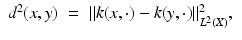
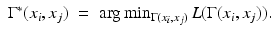
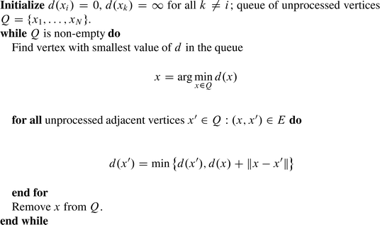
Unfortunately, the graph distance d L is an inconsistent approximation of d X , in the sense that d L usually does not converge to d X when the sampling becomes infinitely dense. This phenomenon is called metrication error, and the reason is that the graph induces a metric inconsistent with d X (Fig. 3). While metrication errors make in general the use of d L an approximation of d X disadvantageous, the Bernstein–de Silva–Langford–Tenenbaum theorem [14] states that under certain conditions, the graph metric d L can be made as close as desired to the geodesic metric d X . The theorem is formulated as a bound of the form
where λ 1, λ 2 depend on shape properties, sampling quality, and graph connectivity. In order for d L to represent d X accurately, the sampling must be sufficiently dense, length of edges in the graph bounded, and sufficiently close vertices must be connected, usually in a non-regular manner.
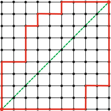
(22)
Fig. 3
Shortest paths measured by Dijkstra’s algorithm (solid bold lines) do not converge to the true shortest path (dashed diagonal), no matter how much the grid is refined (Reproduced from [25])
Fast Marching
Eikonal Equation
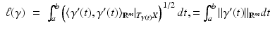
An alternative to computation of a discrete metric on a discretized surface is the discretization of the metric itself. The distance map d(x) = d X (x 0, x) (Fig. 4) on the manifold can be associated with the time of arrival of a propagating front traveling with unit speed (illustratively, imagine a fire starting at point x 0 at time t = 0 and propagating from the source). Such a propagation obeys the Fermat principle of least action (the propagating front chooses the quickest path to travel, which coincides with the definition of the geodesic distance) and is governed by the eikonal equation
where ∇ X is the intrinsic gradient on the surface X. Eikonal equation is a hyperbolic PDE with boundary conditions d(x 0) = 0; minimum geodesics are its characteristics. Propagation direction is the direction of the steepest increase of d and is perpendicular to geodesics.
(23)
Fig. 4
Distance map measured on a curved surface. Equidistant contours from the source located at the right hand are shown (Reproduced from [25])
Since the distance map is not everywhere differentiable (in particular, at the source point), no solution to the eikonal equation exists in the classical sense, while there exist many non  functions satisfying the equation and the boundary conditions. Among such functions, the largest d satisfying the boundary conditions and the inequality
at every point where ∇ X d exists is called the viscosity solution [42]. The viscosity solution of the eikonal equation always exists and is unique, and its value at a point x coincides with d X (x, x 0). It is known to be monotonous, i.e., not having local maxima.
functions satisfying the equation and the boundary conditions. Among such functions, the largest d satisfying the boundary conditions and the inequality(24)
Triangular Meshes
A family of algorithms for finding the viscosity solution of the discretized eikonal equation by simulated wavefront propagation is called fast marching methods [63, 100, 112]. Fast marching algorithms can be thought of as continuous variants of Dijkstra’s algorithm, with the notable difference that they consistently approximate the geodesic metric d X on the surface.
The general structure of fast marching closely resembles that of Dijkstra’s algorithm with the main difference lying in the update step. Unlike the graph case where shortest paths are restricted to pass through the graph edges, the continuous approximation allows paths passing anywhere in the simplicial complex. For that reason, the value of d(x) has to be computed from the values of the distance map at two other vertices forming a triangle with x. In order to guarantee consistency of the solution, all such triangles must have an acute angle at x. Obtuse triangles are split at a preprocessing stage by adding virtual connections to nonadjacent vertices.
Given a triangle (x, x 1, x 2) with known values of d(x 1) and d(x 2), the goal of the update step is to compute d(x). The majority of fast marching algorithms do so by simulating the propagation of a planar wavefront in the triangle. The wavefront arrival time to x 1 and x 2 is set to d(x 1) and d(x 2), from which the parameters of the wave source are estimated. Generally, there exist two solutions for d(x) consistent with the input, the smallest corresponding to the wavefront first arriving to x and then to x 1 and x 2


Related posts:

Stay updated, free articles. Join our Telegram channel
Full access? Get Clinical Tree
