Jet Flow Imaging
Mark Doyle
WHY STUDY JET FLOW?
The presence of jet flow is always associated with pathology. However, simple identification of jet flow is not sufficient to adequately characterize the pathology, including stenotic and regurgitant valves. To be of clinical value, the jet flow must be quantitatively characterized to allow grading or staging the pathology.
JET FLOW FIELD FACTS
While jet flow velocities can be high (in excess of 5 m per second) the acceleration terms can be extremely high (in the range 10 to 200 m per s2). Although it is not common to characterize jets by their acceleration terms, these terms can have a dramatic impact on the accuracy of phase contrast-magnetic resonance (PC-MR). Close to the jet origin the flow field is not turbulent but has a core of laminar flow. As the jet progresses into the static or counter flowing blood, regions of eddy flow develop, which gradually encroach on the laminar jet core and eventually degrade it into turbulent flow (see Fig. 33-1). Depending on the flow conditions, the transition from laminar to turbulent flow may occur over a relatively short distance or may extend quite far into the vessel or chamber.
TWO COMPONENTS OF FLOW
While a high velocity jet is an obvious manifestation of pathology and appears distal to it, the convergent flow field is found proximal to the stenotic site. In vivo, owing to the confined structures of the heart, the jet may encounter a vessel or chamber wall after traversing a very short distance and therefore the jet may not have an opportunity to develop the flow field characteristic of “free jets”. However, just past the stenotic origin, the jet flow will converge, and at this point it is still characterized by laminar flow. The region of maximal convergence is termed the vena contracta. A free jet can ideally be characterized by measuring flow in only the direction along the jet.
In the convergent zone proximal to the jet, a complex three-dimensional (3D) distribution of low velocity flow is found. In the convergent zone, we ideally require measurement of all three velocity directions to characterize flow conditions. However, assumptions can be made to reduce the flow problem to a 1D case, but these assumptions are often incorrect, because they may oversimplify the situation. To fully characterize flow in the convergent zone, it is desirable to quantify velocity in all three directions for each plane visualized. These separate flow components can be visualized as individual components, but to get a more comprehensive view, quiver plots can be used to combine the two in-plane components, for example, left-right and vertical, into one intuitive image format. Using quiver plots, eddy currents can be visualized breaking off the tip of the fully develop jet.
JET ONSET
The onset of jet flow is typically very sudden, and for a jet that develops in <40 milliseconds, it can be appreciated that even with a frame rate of 7 milliseconds (a typical lower limit of scanner performance) only a few frames will capture jet onset. Consider that a temporal resolution of 20 frames per cycle (a more typical performance level) corresponds to 50 milliseconds per frame, and in this instance, onset of jet flow through maturity would be completely missed or blurred into one time frame.
VELOCITY VERSUS ACCELERATION
While jet velocities can be high (1 to 10 m per second), high velocities do not pose a problem for
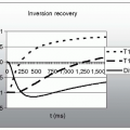
PC-MR. The problem for PC-MR is the high accelerations that are present in jet flow. In Fig. 33-2, we plot velocity and acceleration on the same graphs to show how they are related to each other for a jet flow waveform. In this example, at peak jet flow, the maximum velocity is approximately 160 cm per second, whereas at the jet origin the maximum velocity is close at 130 cm per second. However, the maximum acceleration is dramatically different between these two locations, being 80 cm per s2 versus 30 cm per s2, respectively. Acceleration is problematic because its presence violates some of the key assumptions inherent in PC-MR:
PC-MR. The problem for PC-MR is the high accelerations that are present in jet flow. In Fig. 33-2, we plot velocity and acceleration on the same graphs to show how they are related to each other for a jet flow waveform. In this example, at peak jet flow, the maximum velocity is approximately 160 cm per second, whereas at the jet origin the maximum velocity is close at 130 cm per second. However, the maximum acceleration is dramatically different between these two locations, being 80 cm per s2 versus 30 cm per s2, respectively. Acceleration is problematic because its presence violates some of the key assumptions inherent in PC-MR:
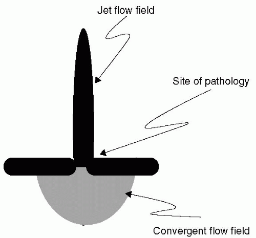 FIGURE 33-1 At the site of a stenosis, two distinct flow patterns are seen: on the proximal side, flow accelerates toward the orifice while only achieving relatively low velocities, and when passing through the orifice it becomes a high-velocity jet. The vena contracta describes the jet region where the cross-sectional area is minimal and the velocity is maximal, and this typically occurs a few millimetres distal to the orifice. |
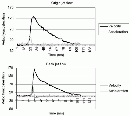 FIGURE 33-2 Simultaneous plots of velocity and acceleration for jet flow at two distinct positions: top panel, just past the jet origin and lower panel, close to the tip of the fully developed jet. Notice the increase in acceleration at the jet tip, although the velocity does not increase substantially between the two points. |
Velocity does not change appreciably over image time for each frame.
Velocity is uniform within each voxel.
Therefore, to accurately measure velocity in jet flow fields, the acquisition needs to satisfy the following two conditions:
High frame rates
High spatial resolution
Conformation to these conditions typically leads to dramatically long scan times.
PROXIMAL FLOW FIELD
The difficulties in imaging jet flow fields using PC-MR have led to a focus on the convergent flow side. The convergent flow field can be quantified using one of two methods:
Proximal iso-velocity surface area (PISA)
Examination of the proximal flow field can be used to quantify the amount of blood passing through a
region of interest such as a stenotic valve. Typically, full 3D visualization of convergent flow is not feasible, and in the simplified PISA approach, only the radius of the isovelocity contour in one direction is measured. Alternatively, the control volume approach can be used, but it requires imaging of several slices, with multiple velocity directions encoded in each slice. For these reasons, quantification of jet flow from an examination of the convergent flow field has not gained widespread acceptance in the magnetic resonance (MR) community. The complexities of this problem make direct visualization of the jet attractive.
region of interest such as a stenotic valve. Typically, full 3D visualization of convergent flow is not feasible, and in the simplified PISA approach, only the radius of the isovelocity contour in one direction is measured. Alternatively, the control volume approach can be used, but it requires imaging of several slices, with multiple velocity directions encoded in each slice. For these reasons, quantification of jet flow from an examination of the convergent flow field has not gained widespread acceptance in the magnetic resonance (MR) community. The complexities of this problem make direct visualization of the jet attractive.
DIRECT JET VISUALIZATION
Assuming that the jet flow can be accurately measured using PC-MR, it is possible to capture this information in one to two slices, capturing either through-plane or in-plane flow. Therefore, direct jet imaging using PC-MR is desirable. However, as indicated earlier, acceleration is problematic for PC-MR and it follows that jet imaging may be inherently prone to artifacts, because commonly applied PC-MR approaches have relatively poor spatial and temporal resolution.
The reason for poor temporal resolution is embedded in the PC-MR scan sequence. Velocity is encoded in the phase of the MR signal by applying specially designed gradient waveforms. These gradients take longer to apply than regular imaging gradients, thereby extending the echo time (TE). Typically, acceleration is not explicitly accommodated in the design of the flow encoding gradients because it would take too long to compensate for, which would further extend the TE. Therefore, it is generally assumed that the gradients are applied sufficiently fast to avoid errors due to acceleration. The assumption is generally true for TEs <4 milliseconds. However, the assumptions break down when multiple lines of k-space are acquired over time and assigned to a single cardiac phase.
ORIGIN OF PROBLEM
Related posts:
Stay updated, free articles. Join our Telegram channel

Full access? Get Clinical Tree


