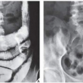
 FIGURE 9.1 Anteroposterior view. (A) For the anteroposterior view of the knee, the patient is supine, with the knee fully extended and the leg in the neutral position. The central beam is directed vertically to the knee with a 5- to 7-degree cephalad angulation. (B) The radiograph in this projection sufficiently demonstrates the medial and lateral femoral and tibial condyles, the tibial plateaus and spines, and both the medial and lateral joint compartments. The patella is seen en face as an oval structure between the femoral condyles. |
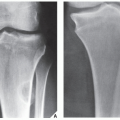
 FIGURE 9.2 Lateral view. (A) For the lateral view of the knee, the patient is lying flat on the same side as the affected knee, which is flexed approximately 25 to 30 degrees. The central beam is directed vertically toward the medial aspect of the knee joint with an approximately 5- to 7-degree cephalad angulation. (B) The radiograph in this projection demonstrates the patella in profile, as well as the femoropatellar joint compartment and a faint outline of the quadriceps tendon. The femoral condyles are seen overlapping, and the tibial plateaus are imaged in profile. Note the slight posterior tilt of the tibial plateaus, which normally measures approximately 10 degrees. |
 FIGURE 9.3 Femoropatellar relationship. The length of the patella and the patellar ligament are approximately equal; normal variability does not exceed 20%. |
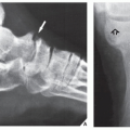
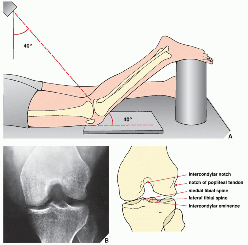 FIGURE 9.4 Tunnel view. (A) For the tunnel (or notch) projection of the knee, the patient is prone with the knee flexed approximately 40 degrees, with the foot supported by a cylindrical sponge. The central beam is directed caudally toward the knee joint at a 40-degree angle from the vertical. (B) The radiograph in this projection demonstrates the posterior aspect of the femoral condyles, the intercondylar notch, and the intercondylar eminence of the tibia. |
 FIGURE 9.5 Sunrise view. (A) For an axial (sunrise) view of the patella, the patient is prone, with the knee flexed 115 degrees. The central beam is directed toward the patella with approximately 15-degree cephalad angulation. (B) The radiograph in this projection demonstrates a tangential (axial) view of the patella. Note the deep position of this structure in the intercondylar fossa. The femoropatellar joint compartment is well demonstrated. |
 FIGURE 9.6 Merchant view. (A) For the Merchant axial view of the patella, the patient is supine on the table, with the knee flexed approximately 45 degrees at the table’s edge. A device keeping the knee at this angle also holds the film cassette. The central beam is directed caudally through the patella at a 60-degree angle from the vertical. (B) On the radiograph obtained in this projection, the articular facets of the patella and femur are well demonstrated. |
 FIGURE 9.7 Sulcus and congruence angles. Two specific measurements can be obtained from the Merchant axial view: the sulcus angle and the congruence angle. The sulcus angle, formed by lines extending from the deepest point of the intercondylar sulcus (a) medially and laterally to the tops of the femoral condyles, normally measures approximately 138 degrees. To determine the congruence angle, the sulcus angle is bisected to establish a reference line (ba), which is drawn to connect the apex of the patella (b) with the deepest point of the sulcus (a). In normal subjects, this line is close to vertical. A second line (ca) is then drawn from the lowest point on the articular ridge of the patella (c) to the deepest point of the sulcus (a). The angle formed by this line and the reference line is the congruence angle. If the lowest point on the patellar articular ridge is lateral to the reference line, then the congruence angle has a positive value; if it is medial to the reference line, as in the present example, then the angle has a negative value. In Merchant’s study, the average congruence angle in normal subjects was −6 degrees (standard deviation [SD], ±11 degrees). (Modified from Merchant AC, Mercer RL, Jacobsen RH, Cool CR. Roentgenographic analysis of patello-femoral congruence. J Bone Joint Surg [Am] 1974;56A:1391-1396.) |
articular cartilage, particularly when subtle chondral or osteochondral fracture is suspected, or when confirmation of the presence or absence of osteochondral bodies in the knee joint is required in suspected osteochondritis dissecans. However, in the evaluation of the menisci, cruciate ligaments, and collateral ligaments, arthrographic examination has been almost completely replaced by MRI.
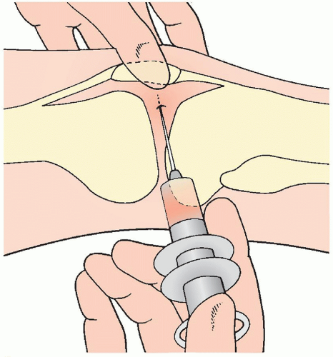 FIGURE 9.8 Arthrography of the knee. For arthrographic examination of the knee, the patient is supine on the radiographic table, with both legs fully extended and in the neutral position. The patella is pulled laterally and rotated anteriorly, and the joint is entered from the lateral aspect at the midpoint of the patella. Before injection of contrast, the joint should be aspirated to avoid dilution of the contrast agent by joint fluid. For a double-contrast study, 40 to 50 mL of room air is injected into the joint, followed by 5 to 7 mL of positive contrast agent (usually 60% diatrizoate meglumine mixed with 0.3 mL of epinephrine 1:1,000, which delays absorption of the contrast). Radiographs are then obtained in the prone position using the spotfilm technique (see Fig. 9.10). |
the cartilage and soft tissues, particularly the menisci and cruciate ligaments. CT used in conjunction with arthrography (computed arthrotomography) is useful in the evaluation of osteochondritis dissecans (see Fig. 9.60C,D) and in detecting nonopaque osteochondral bodies in the knee joint.
 FIGURE 9.9 Tibial plateau. In the topography of the tibial plateau, the medial meniscus is a C-shaped fibrocartilaginous structure with anterior horn attached anteriorly to the intercondylar eminence of the tibia and with posterior horn inserted into the intercondylar area in front of the attachment of the posterior cruciate ligament. The anterior horn of the lateral meniscus, which is an O-shaped structure, is attached in front of the lateral intercondylar tubercle, and the posterior horn inserts medially into the lateral intercondylar tubercle, in front of the attachment of the posterior horn of the medial meniscus. |
 FIGURE 9.10 Arthrography of the knee. Multiple spot films obtained during arthrographic examination of the knee demonstrate the normal appearance of the medial (A-C) and lateral (D,E) semilunar cartilages. The contrast-outlined margins of the medial meniscus show its triangular shape. The posterior horn (A) is longer than the body (B) and the anterior horn (C), and the free edge of the meniscus is sharply pointed. Features of the normal lateral meniscus include the gap of the popliteal hiatus, which separates the meniscus from the joint capsule (D). The posterior horn reattaches to the capsule more posteriorly (E). No contrast should be seen within the substance of any aspect of the menisci. |
 FIGURE 9.11 The cruciate ligaments. In the topography of the cruciate ligaments of the knee, the ACL arises on the medial surface of the lateral femoral condyle at the intercondylar notch (A) and attaches on the anterior portion of the intercondylar eminence of the tibia (C) (see also Fig. 9.9). The posterior cruciate ligament originates on the lateral surface of the medial femoral condyle within the intercondylar notch (B) and inserts on the posterior surface of the intercondylar eminence (D) (see also Fig. 9.9). Neither cruciate ligament is attached to the tibial tubercles. |
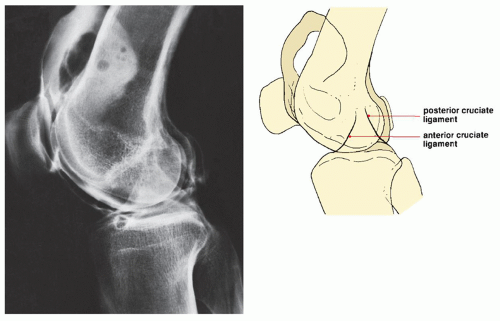 FIGURE 9.12 Arthrography of the cruciate ligaments. Double-contrast arthrogram of the knee demonstrates the normal appearance of the cruciate ligaments. Note the angle formed by their projectional intersection and their taut appearance. Each ligament can be traced from its origin in the femur to its insertion in the tibia. The boundaries of the cruciate ligaments are sharply outlined because the contrast medium coats their synovial reflexions. The cruciate ligaments are extrasynovial structures; only the anterior surface of the ACL and the posterior surface of the posterior cruciate ligament are covered by synovium. |
 FIGURE 9.13 Appearance of normal menisci on MRI. (A) Anterior and posterior horns of the medial meniscus as seen on sagittal T2*-weighted MPGR sequence (flip angle 30 degrees). (B) Anterior and posterior horns of the lateral meniscus as seen on sagittal T2*-weighted MPGR sequence (flip angle 30 degrees). (C) Body of the medial meniscus as seen on sagittal spin echo T1-weighted sequence. (D) Anterior and posterior horns of the lateral meniscus as seen on sagittal spin echo T1-weighted sequence. (E) Schematic representation of topography of the medial and lateral menisci and surrounding structures as seen in the midplane of the coronal MRI. (Modified from Firooznia H, Golimbu C, Rafii M. MR imaging of the menisci: fundamentals of anatomy and pathology. Magn Reson Imaging Clin N Am 1994;2:325-347.) |
 FIGURE 9.14 Cruciate ligaments. Spin echo MR images of the normal cruciate ligaments. (A) Sagittal proton density-weighted image demonstrates the anterior margin of the ACL, straight and well defined, representing the anteromedial bundle; the posterior margin is ill-defined because of the oblique orientation of the ligament and it represents the posterolateral bundle. (B) Oblique coronal T2-weighted image depicts the ACL from the origin in the lateral femoral condyle to the insertion in the tibia (arrows). (C) The posterior cruciate ligament is seen in its entirety, in one sagittal image, from the femoral to the tibial attachments. Observe the small bulge anteriorly produced by the anterior meniscofemoral ligament (arrow). (D) In this sagittal section, the anterior meniscofemoral ligament of Humphrey is very prominent, simulating a loose body or meniscal fragment (arrow). (E) Here, meniscofemoral ligaments, both anterior (Humphrey) and posterior (Wrisberg), are prominent. |
 FIGURE 9.15 Collateral ligaments. (A) Coronal T2-weighted fat-saturated MR image of the normal medial collateral ligament. The superficial fibers of the medial collateral ligament are well defined in this section through the intercondylar notch (arrows). The insertion of the posterior cruciate ligament in the inner aspect of the medial femoral condyle is well demonstrated. The menisci are seen as small triangles of low signal intensity. (B) Coronal T2-weighted fat-saturated image demonstrates the superficial (long arrows) and deep (arrowheads) fibers of the medial collateral ligament. Note the deep crural fascia (short arrow) and the tibial arm of the semimembranosus tendon (T). (C,D) Coronal T2-weighted fat-saturated images of the lateral (fibular) collateral ligament (arrow). On this posterior sections, note the meniscofemoral ligament, which extends from the posterior horn of the lateral meniscus to the inner surface of the medial femoral condyle (arrowheads). The lateral and medial menisci and posterior cruciate ligament are well demonstrated. |
local central depression (type II) and local split depression (type III) fractures occur (Fig. 9.25). Total depression fractures (type IV), which are more commonly seen in the medial tibial plateau because of its anatomic configuration (absence of the fibula), are characterized by the lack of comminution of the articular surface. Type V fractures in the Hohl classification, which are infrequently encountered, are local split fractures without central depression involving the anterior or posterior aspects of the tibial plateau. Comminuted fractures involving both tibial plateaus and having a Y or T configuration (type VI) usually result from vertical compression, such as a fall on the extended leg (Fig. 9.26). Types III and VI are frequently associated with fracture of the proximal fibula. In our institution, we use the Schatzker classification of tibial plateau fractures which, similar to the Hohl classification, arranges tibial plateau fractures into VI types but according to involvement of the medial or lateral plateau (Fig. 9.27).
TABLE 9.1 Checklist for Evaluation of Magnetic Resonance Imaging of the Knee | ||||||||||||||||||||||||||||||||||
|---|---|---|---|---|---|---|---|---|---|---|---|---|---|---|---|---|---|---|---|---|---|---|---|---|---|---|---|---|---|---|---|---|---|---|
| ||||||||||||||||||||||||||||||||||
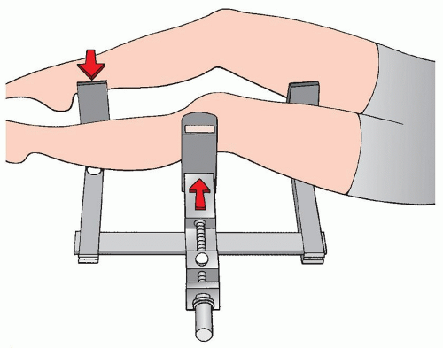 FIGURE 9.16 Valgus stress. For a stress film of the knee evaluating the medial collateral ligament, the patient is supine, with the knee flexed approximately 15 to 20 degrees. The leg is placed in the device, and the pressure plate is applied against the lateral aspect of the knee. (The arrows show the direction of the applied stresses.) Radiographs are then obtained in the anteroposterior projection (see Fig. 9.83B). |
 FIGURE 9.17 Anterior-drawer stress. For a stress film of the knee evaluating the ACL, the patient is placed in the device on his or her side, with the knee flexed 90 degrees. The pressure plate is applied against the anterior aspect of the knee. (The arrows show the direction of the applied stresses.) Radiographs are then obtained in the lateral projection. |
TABLE 9.2 Standard and Special Radiographic Projections for Evaluating Injury to the Knee | ||||||||||||||||||||||||||||||||||||||||||||||||||||||||||||||||
|---|---|---|---|---|---|---|---|---|---|---|---|---|---|---|---|---|---|---|---|---|---|---|---|---|---|---|---|---|---|---|---|---|---|---|---|---|---|---|---|---|---|---|---|---|---|---|---|---|---|---|---|---|---|---|---|---|---|---|---|---|---|---|---|---|
| ||||||||||||||||||||||||||||||||||||||||||||||||||||||||||||||||
TABLE 9.3 Ancillary Imaging Techniques for Evaluating Injury to the Knee | |||||||||||||||||||||||||||||||||||||||||
|---|---|---|---|---|---|---|---|---|---|---|---|---|---|---|---|---|---|---|---|---|---|---|---|---|---|---|---|---|---|---|---|---|---|---|---|---|---|---|---|---|---|
| |||||||||||||||||||||||||||||||||||||||||
 FIGURE 9.18 Spectrum of radiologic imaging techniques for evaluating injury to the knee. The radiographic projections or radiologic techniques indicated throughout the diagram are only those that are the most effective in demonstrating the respective traumatic conditions. #Almost completely replaced by CT. AP, anteroposterior; CT, computed tomography. |
 FIGURE 9.19 Classification of distal femur fractures. Fractures of the distal femur can be classified according to the site and extension of the injury as supracondylar, condylar, and intercondylar fractures. |
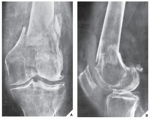 FIGURE 9.20 Supracondylar fracture. A 58-year-old man was injured in a motorcycle accident. Anteroposterior (A) and lateral (B) radiographs of the knee demonstrate a comminuted supracondylar fracture of the distal femur. The extension of the fracture lines and the position of the fragments can be assessed adequately on these standard studies. |
 FIGURE 9.21 Supracondylar fracture. A 22-year-old racing car driver was injured in an accident on the track. (A) Anteroposterior view of the right knee shows a comminuted fracture of the distal femur. Tomography was performed, and sections in the anteroposterior (B) and lateral (C) projections demonstrate intraarticular extension of the fracture lines, with split of the condyles and posterior displacement of the distal fragments. The multiple comminuted fragments can be localized. |
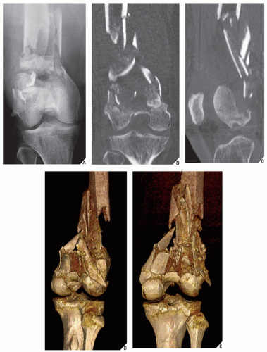 FIGURE 9.22 CT and 3D CT of supracondylar fracture. A 54-year-old woman was injured in a motor vehicle accident. (A) Anteroposterior radiograph of the right knee shows markedly comminuted supracondylar fracture of the femur. (B,C) Coronal and sagittal reformatted CT images show displacement of various fracture fragments. 3D CT reconstructed images, (D) oblique and (E) viewed from the posterior aspect, depict the position and orientation of displaced fracture fragments in more comprehensive fashion. |
 FIGURE 9.23 The Hohl classification of fractures of the tibial plateau. (Modified from Hohl M. Tibial condylar fractures. J Bone Joint Surg [Am] 1967;49A:1455-1467.) |
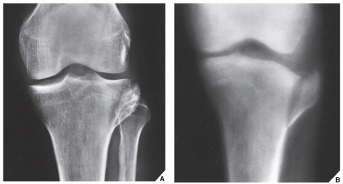 FIGURE 9.24 Fracture of the tibial plateau. A 30-year-old man was hit by a car while he was crossing the street. Anteroposterior radiograph (A) and tomogram (B) show a split fracture of the lateral tibial plateau (Hohl type I). |
 FIGURE 9.25 Fracture of the tibial plateau. Anteroposterior radiograph of the knee shows the appearance of a tibial plateau fracture, which is a combination of wedge and central depression fractures involving the lateral tibial condyle (Hohl type III). |
 FIGURE 9.26 Fracture of the tibial plateau. Anteroposterior radiograph (A) and lateral tomogram (B) demonstrate the characteristic appearance of the Y-type bicondylar tibial fracture (Hohl type VI). |
 FIGURE 9.27 The Schatzker classification of fractures of the tibial plateau. (Modified from Koval JK, Helfet DI. Tibial plateau fractures: evaluation and treatment. J Am Acad Orthop Surg 1995;3:86-93.) |
 FIGURE 9.28 Fracture of the tibial plateau. While crossing the street, a 38-year-old woman was struck by a car. Anteroposterior (A) and lateral (B) radiographs show substantial joint effusion, but the fracture line is not clearly seen. (C) Cross-table lateral view demonstrates the FBI sign, indicating intraarticular extension of the fracture. |
 FIGURE 9.29 CT of fracture of the tibial plateau. A 23-year-old man was injured in a motorcycle accident. The conventional radiographs of the right knee (not shown here) demonstrated a fracture of the tibial plateau. (A) Axial CT section through the proximal tibia shows a comminuted fracture of the medial tibial plateau. (B) Sagittal reformatted image shows that the anterior part of the plateau is mainly affected. (C) Coronal reformatted image demonstrates comminution and depression. (D) Anterior view of the 3D reconstructed image in addition to depression of the medial anterior tibial plateau shows associated fracture of the proximal fibula. (E) Bird’s eye view of the 3D reconstructed image shows the spatial orientation of the fracture lines. |
 FIGURE 9.30 CT of fracture of the tibial plateau. A 22-year-old man fell down from a tall ladder and injured his right knee. The conventional radiographs demonstrated fracture of the tibial plateau. (A) Coronal reformatted CT scan shows extension of the lateral tibial plateau fracture into the tibial shaft. (B) Posterior view of the 3D reconstruction shows the fracture line, but the interfragmental split is not well demonstrated. (C) Anterior view of the 3D reconstruction shows the split better. (D) Bird’s eye view of the 3D CT scan effectively demonstrates the details of the split and comminution of the tibial plateau. |
or comminuted (Fig. 9.39). In the most commonly encountered patellar injury, seen in 60% of cases, the fracture line is transverse or slightly oblique, involving the midportion of the patella. In evaluation of such injury, it is important to recognize what has been called the bipartite or multipartite patella. This anomaly represents a developmental variant of the accessory ossification center or centers of the superolateral margin of the patella and should not be mistaken for a fracture (Fig. 9.40). CT may help distinguish this developmental anomaly from patellar fracture. As an aid to avoid misdiagnosing a bipartite or multipartite patella as a fracture, it is important to keep in mind that the accessory ossification centers are invariably in the upper lateral quadrant of the patella and, if the apparent fragments are put together, they do not form a normal patella. Fracture fragments, however, form a normal patella if they are replaced. Injury to the patella is usually sufficiently demonstrated on the overpenetrated anteroposterior and lateral radiographs of the knee (Figs. 9.41, 9.42, 9.43).
 FIGURE 9.31 CT of fracture of the tibial plateau. Coronal (A) and sagittal (B) CT reformatted images show a Hohl type III (displaced, local spit depression) fracture of the lateral tibial plateau. (C) 3D reconstructed image (posterior view) more realistically depicts the features of this injury. |
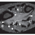
 FIGURE 9.32 MRI of fracture of the tibial plateau. (A) T2-weighted (spin echo, TR 2000/TE 80 msec) coronal image shows a broad-based band of low signal intensity traversing the lateral tibial plateau (long arrows). Extensive soft-tissue edema is seen superficial to the iliotibial band (small arrows). (B) Proton density-weighted (spin echo, TR 2000/TE 20 msec) sagittal image shows central localized depression of the tibial plateau (arrow). The degree of comminution and depression is well depicted. (From Bloem JL, Sartoris DJ, eds. MRI and CT of the musculoskeletal system. A text-atlas. Baltimore: Williams Wilkins; 1992.) |
 FIGURE 9.33 MRI of fracture of the tibial plateau. (A) Coronal gradient echo (MGPR) image shows a tibial plateau fracture (arrowheads). (B) Sagittal gradient echo (MGPR) image demonstrates the anterior extension of the fracture and evulsion of the tibial spines (arrowheads). (From Berquist TH, ed. MRI of the musculoskeletal system, 3rd ed. Philadelphia: Lippincott-Raven Publishers; 1997.)
Related posts: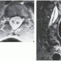 Radiologic Evaluation of Skeletal Anomalies Radiologic Evaluation of Skeletal Anomalies
 Inflammatory Arthritides Inflammatory Arthritides
 Benign Tumors and Tumor-like Lesions II: Lesions of Cartilaginous Origin Benign Tumors and Tumor-like Lesions II: Lesions of Cartilaginous Origin
 Benign Tumors and Tumor-Like Lesions III: Fibrous, Fibroosseous, and Fibrohistiocytic Lesions Benign Tumors and Tumor-Like Lesions III: Fibrous, Fibroosseous, and Fibrohistiocytic Lesions
 Anomalies of the Upper and Lower Limbs Anomalies of the Upper and Lower Limbs
 Upper Limb III: Distal Forearm, Wrist, and Hand Upper Limb III: Distal Forearm, Wrist, and Hand
Stay updated, free articles. Join our Telegram channel
Full access? Get Clinical Tree
 Get Clinical Tree app for offline access

|