Medical Image Computing for Oncology: Review and Clinical Examples

Fig. 6.1

Registration-based skull stripping method. (a) Original image to be processed; (b) the template image; (c) the segmented brain region of the template image; (d) overlapping the brain region onto the original image [41]

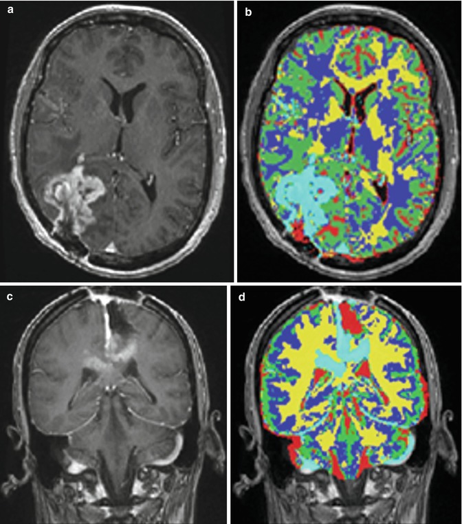
Fig. 6.2

Some examples of tumor segmentation results after FAST. (a, c) Input images; (b, d) FAST segmentation results [41]

To reduce the false-positive spots, we developed a T2 mapping method to remove them. As shown in Fig. 6.3b, the T2-weighted image (Fig. 6.3a) was first registered onto the T1-weighted image with initial segmentation of FAST overlap. A low-bound intensity thresholding was then applied to the registered T2-weighted image, and only high-intensity regions covering all the segmented tumor regions but not the false-positive regions were kept. Combining the T1 and T2 segmentation results and performing morphological shape corrections, we obtained the final automatic tumor segmentation. Then, the tumor can be automatically selected by using morphological operations. Therefore, regions with small volumes or flat shapes were deleted by applying 3D open operation. If the tumor seed points are provided, a region grow operation will be performed to further remove false-positive regions. Figure 6.3e illustrates the final automatic segmentation of the tumor.

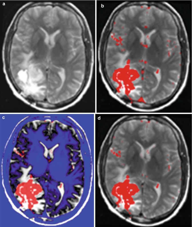
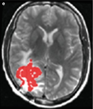
Fig. 6.3

An illustration of the combined T1 and T2 segmentation. (a) T2 image registered onto T1 image; (b) overlaying the segmentation result from T1 image onto T2 image; (c) thresholding T2 image (blue shows the ROI filtered out); by adjusting the threshold, we can eliminate the enhanced big vessels close to the tumor; (d) after applying T2 thresholding, the majority of false-positive spots were removed; and (e) other isolated spots are removed using morphological operations [41]

After automatic segmentation, level-set-based segmentation can be further performed to interactively refine the results by visualization and manual correction [43]. These tasks were accomplished by embedding ITK-SNAP into our software pipeline. ITK-SNAP is a software application used to segment structures in 3D medical images. It provides semiautomatic segmentation using level set methods, as well as manual delineation and image navigation.

Finally, after the segmented tumor result is accepted, the tumor volume, tumor center point location, and the overlapping of the segmented tumor region on the original images were automatically generated in the original DICOM format using a new series number. According to the current neuroradiology workflow, the new data series can be uploaded to a PACS server so that radiologists can interpret the images of GBM patients by referring to the segmentation results.

6.2.3 Results

All the GBM tumor patient cases were processed using the proposed AFINITI pipeline. Of all 26 cases, 24 were visually inspected and found satisfactory by the participating neuroradiologists, and two cases were further refined using the second step, namely, level-set-based refinement. The average time for the two cases using level-set-based refinement was approximately 4 min. Quantitative measurements from manual segmentation and from AFINITI were compared. Denoting the results of AFINITI as set A and those of manual segmentation as M, the ratio of the intersection versus the union, i.e., |A∩M|/|A∪M|, was calculated. Figure 6.4 shows the correlation between AFINITI and manual segmentation, and the Pearson correlation coefficient for all the 26 cases is 0.96.

Fig. 6.4

Correlation of the segmentation results [41]

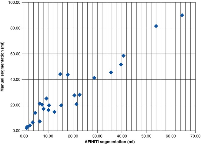
Figure 6.5 shows the original images, the manual and AFINITI segmentation results, and the overlapping images of these two cases. The tumor sizes measured from AFINITI were generally smaller than those obtained from manual segmentation, suggesting that human raters tend to over-segment tumor. During manual selection of the tumor regions, the bright enhanced regions were marked while the small dark regions inside and close to the tumor boundary were not selected. Therefore, although AFINITI results generated a more detailed boundary of the tumor (Fig. 6.5c), the volumes were slightly smaller. Considering the Pearson correlation coefficient between AFINITI and manual results, they are highly correlated, suggesting comparable performance for the proposed automatic tumor segmentation pipeline.

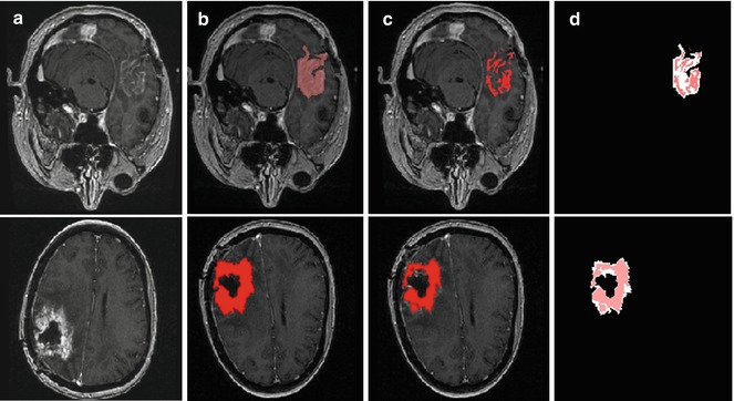
Fig. 6.5

Difference between manual and semiautomatic segmentations: (a) original image; (b) manual segmentation; (c) semiautomatic segmentation; (d) difference between manual segmentation (background white shape) and semiautomatic segmentation (highlighted red shape) [41]

We also compared AFINITI segmentation against voxel-based segmentation (FSL FAST). Because the segmentation results of the voxel-based segmentation lacked spatial continuity (see Fig. 6.2d for example), they were further processed with tumor selection and morphological operation for the comparison. No manual interaction was involved in any of the 26 cases for the FAST algorithm. The student T-Test of the Jaccard indexes of AFINITI and voxel-based results (p-value = 0.0071) showed the advantage of AFINITI. To further evaluate the agreement and systematic differences between segmentation methods and manual segmentation, the Bland-Altman plots of the volume measures between AFINITI and manual results, and between FAST and manual results, were shown in Fig. 6.6. The horizontal axis is the average of the volume measure, and the vertical axis indicates the difference between manual and automatic measures (manual – automatic). It can be seen that FAST generated relatively large errors as compared to AFINITI. Meanwhile, as stated in the above discussions, AFINITI tends to yield less volume because of the detailed segmentation of enhanced tumor regions (see Fig. 6.5 for details).

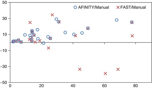
Fig. 6.6

Bland-Altman plots of the volume measures between AFINITI and manual results and between FAST and manual results, respectively [41]

Finally, it is worth noting that the automatic process of AFINITI took approximately 20 min for each dataset using a workstation with 1.86G Hz Intel Core 2 CPU and 2 GB RAM, and the average interactive refinement process took approximately 4 min of operator time. In contrast, the time required for manual segmentation of the dataset varied considerably, depending on the attributes of the tumor, ranging from 30 to 90 min. In the proposed clinical workflow, the scanned data would be first automatically routed to the AFINITI workstation for data processing prior to study interpretation, and the segmented AFINITI output would be transferred as a new additional series of images onto the PACS server along with the quantitative measurement of the tumor. The interpreting radiologists would examine the overlays to confirm the accuracy of automatic segmentation and incorporate the volumetric output into the clinical report as part of the standard workflow.

Evaluation of the software by comparison of volumetric output with manual segmentation of the same clinical dataset showed a significant linear correlation and high degree of overlapping. Although the process time used for manual operation was not rigorously evaluated, use of the system reduced clinical operator time required for segmentation and quantitation from approximately 30–90 min per case to less than 4 min in the roughly 8 % of cases that required correction and to less than 1 min in the majority of cases where the AFINITI output did not require correction. It is not clear how the average processing time using software based on the AFINITI method would compare with currently available commercial software for assisted manual segmentation. Clearly, recently released commercial tools would be expected to substantially decrease operator time compared with the open-source tools used in this study, but it seems unlikely that even these tools could achieve a lower average operator time for segmentation and quantitation than what the AFINITI method provides. The software package was evaluated using the typical clinical MRI data, although ideally the robustness of the algorithm can be tested with different protocols. Due to the availability of manual results, we did not compare the accuracy for different groups of protocols. This could be a future work by using clinical studies from multiple scanners.

Nevertheless, the fraction of cases that require operator correction are clearly an area that requires further development, possibly with incorporation of additional data types. In addition, the processing time of 20 min is significant, although, since this is proposed to occur offline prior to expert interpretation, it is not a critical problem for current diagnostic imaging workflow. This processing speed and the user-friendliness of the graphical interface need to be further improved for full clinical translation of the methods presented as will production of FDA-approved software tools. Both of these improvements and full translation will require product development resources that are beyond the scope of our lab, so we are releasing the AFINITI software pipeline free of charge on our website http://www.cbi-tmhs.org/AFINITI/ in the hope that other groups will be able to extend our work and that its availability will motivate the development of fully translatable clinical tools.

An additional significant weakness is that 2D input data was used for the T2-weighted image analysis, which has large separation between slice thickness (5 ~ 6 mm). 3D T2-weighted whole brain image data was not available routinely at the time that the initial datasets were acquired for this study, but because of rapid progress in 3.0 T MRI, they are now routinely available for clinical brain imaging. Adaptation of the software to perform segmentation on high-resolution 3D T2-weighted image datasets is important because inclusion of such datasets would allow automated assessment of infiltrative progression as required for use of the recently proposed RANO criteria for brain tumor follow-up and would allow automated computation of recently proposed image metrics such at rNTR that may be more predictive of patient outcome [9].

The automatic tumor delineation pipeline could be applied in clinics by first automatically routing the scanned data to the AFINITI workstation for automatic data processing prior to study interpretation. After this, the segmented AFINITI output will be superimposed on the original MRI images, and new images are generated with new series numbers under the same patient ID. The data are then transferred onto the PACS server along with the quantitative measurement of the tumor. The interpreting radiologists would examine the overlay images together with the original sequences for diagnosis and for incorporating the volumetric measures into the clinical report as part of the standard workflow.

Currently, after segmentation, quantitative measures of tumor can be obtained, relieving the tedious work load for manual segmentation. The quantitative measures can be used in a follow-up study that precisely gives the temporal changes for tumor evaluation. In the long run, we foresee that computational image analysis could provide more detailed measures after segmentation, such as heterogeneity measures, transition from enhanced tumor to necrosis, and transition from enhanced tumor to edema. Generally, in contrast-enhanced MR images, GBM consists of enhancing tumor, necrosis, and non-enhancing tumor, including edema. In multimodal MR, enhanced tumor can be clearly seen from T1 post-contrast images but non-enhanced tumor often overlaps with edema by visual assessment. Quantitative segmentation is thus important to segment GBM in detail and to help neuroradiologists determine the tumor margin and determine the aggressiveness of GBM.

6.2.4 Improvement of Level Set Segmentation to 4D

The GBM segmentation can also be improved for semiautomatic segmentation of brain tumor from T1 images in serial MR images, called prior information constrained evolution (PICE) [43]. First, PICE uses a level set framework not only based on image gradient but also based on intensity distribution inside and outside brain tumor, which is estimated using nonparametric density estimation. Then, we show that this framework can be extended to tumor segmentation for longitudinal images so that the prior distribution consists of the intensity distribution in the current image can also contain information obtained from other time-point images. For a single-time-point image, the evolution of the level set is based on the image gradient and the intensity distribution of the current image. For serial images, the prior information obtained from the images of the same patient at other time points is added to the level set evolution for more longitudinally consistent segmentation. In experiments we compared PICE with the traditional level set method in 3-D. In addition, we also illustrate that it can be easily extended to 4-D images, which facilitates follow-up studies of brain tumor treatments. Using longitudinal glioblastoma data from five patients, we showed the advantages of the proposed algorithm.

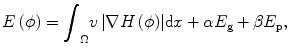
The proposed method aims to segment brain tumor semiautomatically from T1-weighted MR brain images. Our approach is a combination of the image gradient information and the image intensity information in the level set formulation. In level set methods, the basic idea is that a contour C can be represented by the zero-level set of a higher dimensional function ϕ : Ω → R in the image domain Ω. The embedding function can be defined as the signed distance function (SDF) with ϕ < 0 inside the contour and ϕ > 0 outside the contour. The contour is propagated by evolving the embedding function ϕ according to an appropriate partial differential equation (PDE). The PDE can be directly derived from the energy function E(ϕ) defined on the space of the image domain.

6.2.4.1 3-D PICE

For tumor segmentation from single-time-point 3-D images, gradient and intensity distribution of brain tumor can be combined in the evolution with the energy function:

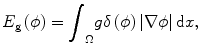
$E\left(\phi \right)={\displaystyle {\int}_{\Omega}v\left|\nabla H\left(\phi \right)\right|}\mathrm{d}x+\alpha {E}_{\mathrm{g}}+\beta {E}_{\mathrm{p}},$

(6.1)

where the first term guarantees a smooth zero-level set function and the second term E _g is the gradient term ensuring that the image gradients along the zero-level set are larger than others. The last term E _p is the intensity prior term used to constrain the intensity distribution inside and outside tumor. The level set function can be calculated by minimizing the energy function E(ϕ). The gradient term E _g is defined as follows:

${E}_{\mathrm{g}}\left(\phi \right)={\displaystyle {\int}_{\Omega} g\delta \left(\phi \right)}\left|\nabla \phi \right|\mathrm{d}x,$

(6.2)

where δ is the Dirac function, g is the boundary indicator function g = 1/1 + | ∇ G ∗ I(x)|², and G is the Gaussian function. I(x) is the image intensity at voxel x. It can be seen that this energy term can be minimized when the zero-level set matches the boundaries in image I. For the prior intensity information, in the Bayesian framework, this can be computed by maximizing the posterior distribution:

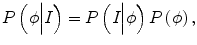
$P\left(\phi \Big|I\right)=P\left(I\Big|\phi \right)P\left(\phi \right),$

(6.3)

where P(I|ϕ) is the conditional distribution of image intensities given the current zero-level set ϕ. P(ϕ) is the shape prior. Because in tumor segmentation the shape prior is unknown, the energy term E _pcan be calculated as

${E}_p=-{\displaystyle {\int}_{\Omega} \log P\left(I\Big|\phi \right)}\mathrm{d}x,$

(6.4)

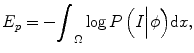
Using the Heaviside step function H(), the energy term ends up with

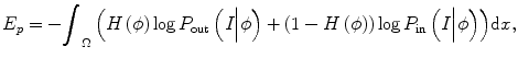
${E}_p=-{\displaystyle {\int}_{\Omega}\left(H\left(\phi \right) \log {P}_{\mathrm{out}}\left(I\Big|\phi \right)+\left(1-H\left(\phi \right)\right) \log {P}_{\mathrm{in}}\left(I\Big|\phi \right)\right)}\mathrm{d}x,$

(6.5)

where P _in(I|ϕ) and P _out(I|ϕ) are the conditional distribution of image intensities inside and outside of the zero-level set function. It can be seen that the difference of this method with other methods is that it combines both boundary information and intensity distribution in one evolution and uses nonparametric density estimation for distribution estimation.

6.2.4.2 4-D PICE

In this section we show that PICE can be easily extended for 4-D tumor segmentation. One of the important applications of tumor segmentation is follow-up study, wherein longitudinal changes are the important measures. Although registration of longitudinal images is necessary for this application, the accuracy is not very important since we only need to establish correspondence of tumor, not the tumor boundaries. Thus the image intensity information of the tumor at different time points can then be used for tumor segmentation. Notice that the tumor shapes can be different and the intensity information might be more consistent. Intuitively our rationale is that by correlating the intensity distribution among different time points, the segmentation criteria tend to be the same at different time points and thus yield relatively stable segmentation results across different time points.

Specifically E _pin Eq. (6.1) needs to consider not only the intensity information from the current time-point image but also the intensity distribution from other time-point images. Therefore, Eq. (6.3) can be rewritten as

$P\left(\phi \Big|I,\tilde{\phi},\tilde{I}\right)=P\left(I\Big|\phi, \tilde{\phi},\tilde{I}\right)P\left(\phi \Big|\tilde{\phi},\tilde{I}\right),$

(6.6)

where $\tilde{\phi}$ and $\tilde{I}$ reflect the segmentation results and the images at other time points. In Eq. (6.6), $P\left(\phi \Big|\tilde{\phi},\tilde{I}\right)$ can be omitted since we do not want to enforce any temporal shape constraints on the longitudinal tumor shapes. However, for the same patient, our rationale is that the intensity information within the brain tumor might be longitudinally similar which can help to improve the longitudinal consistency in segmenting tumors in different time points. Based on this observation, Eq. (6.6) becomes

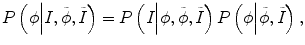
$P\left(I\Big|\phi, \tilde{\phi},\tilde{I}\right)\simeq P\left(I\Big|\phi \right)P\left(I\Big|\tilde{\phi},\tilde{I}\right),$

(6.7)

where the constraints of image information from other time-point images can be reflected by the prior probability $P\left(I\Big|\tilde{\phi},\tilde{I}\right)$ and P(I|ϕ) is the same as Eq. (6.3). The prior probability is divided into two parts: inside the tumor and outside the tumor or ϕ. We use the histograms of the inside and outside as the prior information obtained from other time-point segmentation results. So $P\left(I\Big|\tilde{\phi},\tilde{I}\right)$ can be written as $P\left(I\Big|\tilde{\phi},\tilde{I}\right)=P\left({h}_{\mathrm{in}},{h}_{\mathrm{out}}\Big|{\tilde{h}}_{\mathrm{in}},{\tilde{h}}_{\mathrm{out}}\right)=P\left({h}_{\mathrm{in}}\Big|{\tilde{h}}_{\mathrm{in}}\right)p\left({h}_{\mathrm{out}}\Big|{\tilde{h}}_{\mathrm{out}}\right)$ , assuming that the two conditional distributions are independent and can be separated. In this work for convenience of calculation, we only consider the histogram inside the tumor, $P\left(I\Big|\tilde{\phi},\tilde{I}\right)=P\left({h}_{\mathrm{in}}\Big|{\tilde{h}}_{\mathrm{in}}\right)$ , since the selection of corresponding regions outside tumor is ad hoc. Thus the energy function E(ϕ) in Eq. (6.1) can be written as

$E\left(\phi \right)=v{\displaystyle {\int}_{\Omega}\left|\nabla H\left(\phi \right)\right|} dx+\alpha {\displaystyle {\int}_{\Omega} g\delta \left(\phi \right)\left|\nabla \phi \right|\mathrm{d}x}-\beta {\displaystyle {\int}_{\Omega}\left( \log \left(P\left(I\Big|\phi \right)\right)+ \log \left(P\left({h}_{\mathrm{in}}\Big|{\tilde{h}}_{\mathrm{in}}\right)\right)\right)}\mathrm{d}x,$

(6.8)

where h _in represents the histogram of image intensity inside the tumor at the current time point and ${\tilde{h}}_{\mathrm{in}}$ is the histogram of image inside $\tilde{\phi}$ at another time point. This term involves the information in other time points and can be calculated as

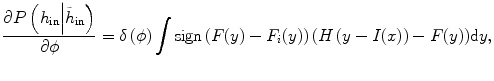
$\frac{\partial P\left({h}_{\mathrm{in}}\Big|{\tilde{h}}_{\mathrm{in}}\right)}{\partial \phi }=\delta \left(\phi \right){\displaystyle \int \mathrm{sign}\left(F(y)-{F}_i(y)\right)\left(H\left(y-I(x)\right)-F(y)\right)}\mathrm{d}y,$

(6.9)

where y is the range of intensity, such as [0,…, 255]. F(y) is the integrate of histogram of image in the current time point. This term ensures that the tumor intensity distributions at different time points for the same patients are similar. Notice that $P\left({h}_{\mathrm{in}}\Big|{\tilde{h}}_{\mathrm{in}}\right)$ can be calculated not only from one image but also from multiple images at different time points.

In order to achieve the proposed algorithm, image registration is necessary for serial images of the same patient. Given a series of MRI images I _n, n = 1, …, N, all the subsequent images were first globally aligned onto the space of the baseline by applying the rigid registration in FLIRT. This is accurate enough to build the correspondence among the tumor regions at different time points.

6.2.4.3 Results

The experiment consists of two parts. One is the segmentation of GBM from single-time-point images. Another one is the serial image segmentation. The dataset contains the MRI image from five patients, and every patient has two time-point images. For each patient, the images are either longitudinal images before resection or those after resection. Currently the proposed PICE does not apply to the longitudinal data containing both images before and after resection. The MRI images of each patient are acquired on a 1.5 T GE signal MR scanner. Images are T1 modality with a high resolution of 256 × 256 × 124 or 192 × 256 × 128. The voxel size is 0.94 × 0.94 × 1.50 mm³.

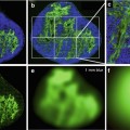
In our experiments, we found that the traditional level set method can derive good results if the tumor intensity is homogeneous, e.g., when the tumor is brighter than the tissues around it, and it did not work well when both bright and dark regions are present in the tumor, i.e., it can’t handle the inhomogeneous tumor due to complexity of edges. In comparison, using the same seed points inside the tumor, the results from PICE show that it can segment tumor well from single-time-point 3-D MRI images, even the intensity of the tumor vary complex. Figure 6.7 gives an example. Quantitatively, for all the ten testing images, compared to the manually marked ground truth, the volumetric ratios of the automatically segmented tumors with respect to the manual tumors are 98.3 ± .2 % for PICE and 87.8 ± 4.7 % for the traditional level set algorithm. It can be seen that PICE obtains very accurate segmentation results and significantly improves the performance of the traditional level set method (p < 0.05).

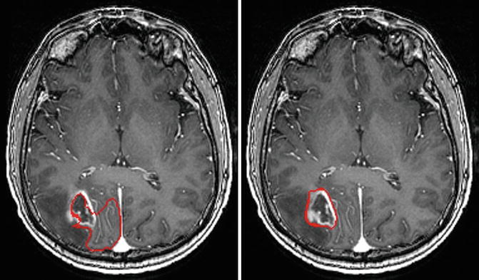
Fig. 6.7

Example of the segmentation results by traditional level set method (left) and PICE (right). The red contour is the boundary of the segmentation result [43]

The PICE algorithm was then used to segment tumor from longitudinal images. Figure 6.8 shows the segmentation results of a patient at different time points using 4-D PICE. Quantitatively, in terms of volumetric ratios of the segmented tumors with respect to the manual results, they are actually very similar to those of the 3-D cases, and we did not find significant differences between them. In fact, the improvement might be in the subtle temporal stability in tumor follow-up study, and two time points are limited to test this factor. More tests will be done after sufficient data are collected.

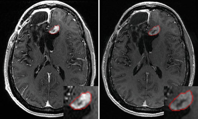
Fig. 6.8

Segmentation results illustrated on globally aligned images. Left is the result at time point 1; right is the result at time point 2 [43]

6.2.5 Concluding Remarks on AFINITI for GBM Applications

We presented an image computing pipeline for GBM segmentation and demonstrated its applicability to clinical data. The software adopts the current state-of-the-art tumor segmentation algorithms and combines the advantages of the traditional voxel-based and deformable shape-based segmentation methods. This provides automatic tumor segmentation based on both T1- and T2-weighted MR brain data, with graphical and numerical output that can be visualized and interactively refined using the embedded GUI based on the ITK-SNAP framework. Finally, the software was incorporated into a conventional PACS-based MRI interpretation workflow. Validation of results using clinical GBM data showed high correlation between the AFINITI results and manual annotation and suggested significant reduction in operator time for performing volumetric quantitation of GBM. The AFINITI pipeline is freely available from our public website (see http://www.cbi-tmhs.org/Projects/AFINITI/).

6.3 Tumor Follow-Up Study: Examples of PET/CT Dual-Modality Imaging

6.3.1 Introduction

Lymphoma is a hematologic malignancy of lymphocyte origin, accounting for approximately 5 % of all cancers in the United States [44]. Classically, lymphomas are classified as Hodgkin’s disease (HD) or non-Hodgkin’s lymphoma (NHL) with several subclassification schemes to describe various cellular, genetic, and clinical subtypes [45]. Treatment for lymphoma is dependent on its type and stage, as well as the age and general clinical status of patients. For most early-stage lymphomas, standard first-line therapy for lymphoma includes chemotherapy with or without radiation therapy [46]. Immunotherapy and hematopoietic stem-cell transplantation have added to the oncologic armamentarium particularly for patients with aggressive or advanced disease. Adoptive immunotherapeutic approaches using genetically modified cytotoxic T lymphocytes (CTL) with engineered tumor-antigen-recognizing receptors have shown promising preclinical and clinical results to date [47–50]. The Epstein-Barr virus (EBV) is known to be associated with a high percentage (up to 40 %) of HD and NHL [51]. Thus, viral-expressed proteins represent highly specific antigen targets. Recently engineered CTLs that recognize an EBV protein, called LMP2, can produce complete responses in HD and NHL patients [52].

Accurate monitoring of patients undergoing adoptive CTL therapy is critical for evaluating response and disease recurrence. The diagnostic gold standard, tissue biopsy, is both invasive and logistically difficult to perform on all patients at specific time intervals. Treatment responses are currently assessed by a canonical approach that integrates clinical examination, laboratory findings, and imaging data. The preferred imaging technique is PET/CT, which combines metabolic information using the positron-emitting sugar analog, [F-18]-fluorodeoxyglucose (FDG), with morphologic changes in tumor size acquired from conventional CT [53–59]. Relative FDG uptake in lesions of active high-grade lymphomas is typically high thus allowing for semiquantitative assessment of disease status [60]. However, interpretation of PET/CT studies is dependent on nonstandardized criteria for assessing relative tumor metabolism and methods for measuring mass lesions, both of which are manually performed and calculated. Moreover, diagnostic PET/CT scans acquired at periodic intervals generate a massive amount of data, which require manual selection of regions of interest (ROI) for comparative and quantitative analyses. Currently clinical investigators are hampered by the absence of validated quantitative methods for evaluating therapy response in a comprehensive format. For example, in assessing longitudinal PET/CT imaging data, oncologists generally refer patients to radiologists or nuclear medicine physicians, who then generate interpretations in their standard reporting format. However, conventional diagnostic reports generally do not describe all detectable lesions, and there is usually no quantitative longitudinal comparison. Furthermore, the presence of the adoptively transferred T cells at disease sites may give false-positive results on PET requiring prolonged follow-up on imaging. Thus there is an urgent need to develop robust methods and tools for quantitative assessment of therapeutic response.

Several methods have been developed to evaluate the treatment response in patients with lymphoma [61–68]. Although computer-aided methods for lymphoma segmentation [69, 70] and longitudinal CT analysis exist [71], these methods apply global affine transformation or pairwise free-form deformable registration for processing longitudinal image data, and there is a lack of longitudinal stability in the quantitative analysis. Traditional pairwise [72, 73] and groupwise [74] image registration algorithms have been used for image alignment; however, the pairwise algorithms warp each image separately and often cause relatively unstable measures of the serial images because no temporal information of the serial images has been used in the registration procedure. Groupwise image registration methods simultaneously process multiple images but consider the images as a group, not a time series. Thus the temporal information has not been used efficiently. For longitudinal images, the relationship between temporally neighboring images is much more important than that of the images with larger time intervals.

In this work the recently developed joint serial image registration and segmentation algorithm for longitudinal CT data [75] is used in the computer-assisted quantitative analysis for lymphoma treatment monitoring. This longitudinal image navigation and analysis (LINA) software tool [76] facilitates the quantitative evaluation of treatment outcomes for lymphoma patients using a computer-assisted serial image analysis approach and automatically constructs the longitudinal correspondences along serial images for each individual patient. In this way, it is possible to automatically determine ROIs in the serial images after defining them at each time point using a semiautomated segmentation algorithm.

Only gold members can continue reading. Log In or Register to continue