Methods in Shape Analysis

[24, 25, 40], boundary contours of objects [31, 44, 67], multiphase objects [83], as well as the morphologies of images [22].

The analysis of a shape space is typically based on a notion of a distance or dissimilarity measure $d(\cdot,\cdot )$ between shapes [10, 31, 50, 51, 54, 67], whose definition frequently takes a variational form. This distance can be used to define an average [26, 67] or a median [4, 28] $\mathcal{S}$ of given shapes $\mathcal{S}_{1},\ldots,\mathcal{S}_{n}$ according to $\mathcal{S} =\mathrm{ argmin}_{\tilde{\mathcal{S}}}\sum _{i=1}^{n}d(\tilde{\mathcal{S}},\mathcal{S}_{i})^{p}$ for p = 1 and p = 2, respectively (cf. section “Elastic Shape Averaging”). Likewise, shape variations can be obtained by a principal component analysis (PCA, cf. section “Elasticity-Based PCA”) or a more general covariance analysis in a way which is consistent with the dissimilarity measure between shapes [11, 16, 26, 68]. From the conceptional point of view, one can distinguish two types of these dissimilarities or distance measures which may be characterized as rather state based or path based, respectively. While the first approach is independent of the notion of paths of shapes, the latter distance definition requires the computation of an optimal, connecting path in shape space. In some cases, both concepts coincide: The Euclidean distance between two points, e.g., can equivalently be interpreted in a state-based manner as the norm of the difference vector or as the length of the shortest connecting path (we shall provide a physical interpretation for each case in section “Recalling the Finite-Dimensional Case”).

The notion of a shape space was already introduced by Kendall in 1984 [39], who considers shapes as k-tuples of points in $\mathbb{R}^{d}$ , endowed with the quotient metric of $\mathbb{R}^{kd}$ with respect to similarity transforms. Often, however, a shape space is just modeled as a linear vector space which is not invariant with respect to shift or rotation a priori. In the simplest case, such a shape space is made up of vectors of landmark positions, and distances between shapes can be evaluated in a state-based manner as the Euclidean norm of their difference. Chen and Parent [12] investigated averages of 2D contours already in 1989. Cootes et al. perform a PCA on training shapes with consistently placed landmarks to obtain priors for edge-based image segmentation [16]. Hafner et al. use a PCA of position vectors covering the proximal tibia to reconstruct the tibia surface just from six dominant modes [35]. Perperidis et al. automatically assign consistent landmarks to training shapes by a nonrigid registration as a preprocessing step for a PCA of the cardiac anatomy [63]. Söhn et al. compute dominant eigenmodes of landmark displacement on human organs, also using registration for preprocessing [73].

As an infinite-dimensional vector space, the Lebesgue-space L ² has served as shape space, where again shape alignment is a necessary preprocessing step. Leventon et al. identify shapes with their signed distance functions and impose the Hilbert space structure of L ² on them to compute an average and dominant modes of variation [43]. Tsai et al. apply the same technique to 3D prostate images [79]. Dambreville et al. also compute shape priors, but using characteristic instead of signed distance functions [19].

A more sophisticated state-based shape space is obtained by considering shapes as subsets of an ambient space with a metric $d(\cdot,\cdot)$ and endowing them with the Hausdorff distance

$\displaystyle{ d_{{\mathrm{H}}}(\mathcal{S}_{1},\mathcal{S}_{2}) =\max \{\sup _{x\in \mathcal{S}_{1}}\inf _{y\in \mathcal{S}_{2}}d(x,y),\sup _{y\in \mathcal{S}_{1}}\inf _{x\in \mathcal{S}_{2}}d(x,y)\} }$

between any two shapes $\mathcal{S}_{1},\mathcal{S}_{2}$ . Charpiat et al. employ smooth approximations of the Hausdorff distance based on a comparison of the signed distance functions of shapes [10]. For a given set of shapes, the gradient of the shape distance functional at the average shape is regarded as shape variation of the average and used to analyze its dominant modes of variation [11]. Frame indifference is mimicked by an inner product that weights rotations, shifts, scalings, and the orthogonal complement to these transformations differently. Charpiat et al. also consider gradient flow morphing from one shape onto another one which can be regarded as a means to obtain meaningful paths even in shape spaces with state-based distance measures.

An isometrically invariant distance measure between shapes (or more general metric spaces) that is also not based on connecting paths is provided by the Gromov–Hausdorff distance, which can be defined variationally as

$d_{GH} (S_1,S_2 ) = \frac{1} {2}\,\mathop {\inf }\limits_{\scriptstyle \phi :S_1 \to S_2 \atop \scriptstyle \psi :S_2 : \to S_1}\,\mathop {\sup }\limits_{\scriptstyle y_i = \phi (x_i ) \atop \scriptstyle \psi (y_i ) = x_i}\,|ds_1 (x_1,x_2 ) - ds_2 (y_1,y_2 )|,$

where $d_{\mathcal{S}_{i}}(\cdot,\cdot )$ is a distance measure between points in $\mathcal{S}_{i}$ . The Gromov–Hausdorff distance represents a global, supremum-type measure of the lack of isometry between two shapes. Memoli and Sapiro use this distance for clustering shapes described by point clouds, and they discuss efficient numerical algorithms to compute Gromov–Hausdorff distances based on a robust notion of intrinsic distances $d_{\mathcal{S}}(\cdot,\cdot )$ on the shapes [50]. Bronstein et al. incorporate the Gromov–Hausdorff distance concept in various classification and modeling approaches in geometry processing [6]. Memoli investigates the relation between the Gromov–Hausdorff distance and the Hausdorff distance under the action of Euclidean isometries as well as L ^p-type variants of the Gromov–Hausdorff distance [49].

In [46], Manay et al. define shape distances via integral invariants of shapes and demonstrate the robustness of this approach with respect to noise.

Another distance or dissimilarity measure which also measures the lack of isometry between shapes can be obtained by interpreting shapes as boundaries of physical objects and measuring the (possibly nonlinear) deformation energy of an elastic matching deformation ϕ between two objects [36, 67]. Since, by the axiom of elasticity, this energy solely depends on the original and the final configuration of the deformed object but not on the deformation path, the elastic dissimilarity measure can clearly be classified as state based (as will be detailed in section “State-Based, Path-Independent Elastic Setup”). This physical approach comes along with a natural linearization of shapes via boundary stresses to perform a covariance analysis [68] and will be presented in section “Elasticity-Based Shape Space.” Pennec et al. define a nonlinear elastic energy as the integral over the ambient space of an energy density that depends on the logarithm of the Cauchy–Green strain tensor $\mathcal{D}\phi ^{T}\mathcal{D}\phi$ [61, 62], which induces a symmetric state-based distance.

Typical path-based shape spaces have the structure of a Riemannian manifold. Here, the strength of a shape variation is measured by a Riemannian metric, and the square root of the Riemannian metric evaluated on the temporal shape variation is integrated along a path of shapes to yield the path length. The length of the shortest path between two shapes represents their geodesic distance $d(\cdot,\cdot )$ . Averages are obtained via the Fréchet mean [30], which was further analyzed by Karcher [38]. There is also a natural linear representation of shapes in the tangent space at the Fréchet mean via the logarithmic map, which enables a PCA.

A Riemannian shape space which might still be regarded as rather state than path oriented is given by the space of polygonal medial axis representations, where each shape is described by a polygonal lattice and spheres around each vertex [87]: Here, the Lie group structure of the medial representation space can be exploited to approximate the Fréchet mean as exponential map of the average of the logarithmic maps of the input. Fletcher et al. perform a PCA on these log-maps to obtain the dominant geometric variations of kidney shapes [26] and brain ventricles [27]. Fuchs and Scherzer use the PCA on log-maps to obtain the covariance of medial representations, and they use a covariance-based Mahalanobis distance to impose a new metric on the shape manifold. This metric is employed to obtain priors for edge-based image segmentation [32, 33].

Kilian et al. compute and extrapolate geodesics between triangulated surfaces of fixed mesh topology, using isometry invariant Riemannian metrics that measure the local distortion of the grid [40]. Eckstein et al. employ different metrics in combination with a smooth approximation to the Hausdorff distance to perform gradient flows for shape matching [24]. Liu et al. use a discrete exterior calculus approach on simplicial complexes to compute geodesics and geodesic distances in the space of triangulated shapes, in particular taking care of higher genus surfaces [45].

An infinite-dimensional Riemannian shape space has been developed for planar curves. Klassen et al. propose to use as a Riemannian metric the L ²-metric on variations of the direction or curvature functions of arc length-parameterized curves. They implement a shooting method to find geodesics [41], while Schmidt and Cremers present an alternative variational approach [70]. Srivastava et al. assign different weights to the L ²-metric on stretching and on bending variations and obtain an elastic model of curves [75]. Michor and Mumford examine Riemannian metrics on the manifold of smooth regular curves [51]. They show the standard L ²-metric in tangent space, leading to arbitrarily short geodesics and hence employ a curvature-weighted L ²-metric instead. Yezzi and Mennucci resolved the problem taking into account the conformal factor in the metric [84]. Sundaramoorthi et al. use Sobolev metrics in the tangent space of planar curves to perform gradient flows for image segmentation via active contours [76]. Michor et al. discuss a specific metric on planar curves, for which geodesics can be described explicitly [52]. In particular, they demonstrate that the sectional curvature on the underlying shape space is bounded from below by zero, which points out a close relation to conjugate points in shape space and thus to only locally the shortest geodesics. Finally, Younes considers a left-invariant Riemannian distance between planar curves by identifying shapes with elements of a Lie group acting on one reference shape [85].

When warping objects bounded by shapes in $\mathbb{R}^{d}$ , a shape tube in $\mathbb{R}^{d+1}$ is formed. Delfour and Zolésio [20] rigorously develop the notion of a Courant metric in this context. A further generalization to classes of non-smooth shapes and the derivation of the Euler–Lagrange equations for a geodesic in terms of a shortest shape tube is investigated by Zolésio in [88].

Dupuis et al. [23] and Miller et al. [53, 54] define the distance between shapes based on a flow formulation in the embedding space. They exploit the fact that in case of sufficient Sobolev regularity for the motion field v on the whole surrounding domain Ω, the induced flow consists of a family of diffeomorphisms. This regularity is ensured by a functional $\int _{0}^{1}\int _{\varOmega }Lv \cdot v\,{\mathrm{d}}x\,{\mathrm{d}}t$ , where L is a higher-order elliptic operator [76, 85]. Geometrically, $\int _{\varOmega }Lv \cdot v\,{\mathrm{d}}x$ is the underlying Riemannian metric, and we will discuss related, path-based concepts in section “Path-Based, Viscous Riemannian Setup.” Under sufficient smoothness assumptions, Beg et al. derive the Euler–Lagrange equations for the diffeomorphic flow field [3]. To compute geodesics between hypersurfaces in the flow of diffeomorphism framework, a penalty functional measures the distance between the transported initial shape and the given end shape. Vaillant and Glaunès [80] identify hypersurfaces with naturally associated two forms and used the Hilbert space structures on the space of these forms to define a mismatch functional. The case of planar curves is investigated under the same perspective by Glaunès et al. in [34]. To enable the statistical analysis of shape structures, parallel transport along geodesics is proposed by Younes et al. [86] as the suitable tool to transfer structural information from subject-dependent shape representations to a single-template shape.

In most applications, shapes represent boundary contours of physical objects. Fletcher and Whitaker adopt this viewpoint to develop a model for geodesics in shape space which avoids overfolding [29]. Fuchs et al. [31] propose a Riemannian metric on a space of shape contours, motivated by linearized elasticity. This metric can be interpreted as the rate of physical dissipation during the deformation of a viscous liquid object [82, 83] and will be elaborated in section “Viscous Fluid-Based Shape Space.”

Finally, a shape space is sometimes understood as a manifold, learned from training shapes, and embedded in a higher-dimensional (often linear) space. Many related approaches are based on kernel density estimation in feature space. Here, the manifold is described by a probability distribution in the embedding space, which is computed by mapping points of the embedding space into a higher-dimensional feature space and assuming a Gaussian distribution there. In general, points in feature space have no exact preimage in shape space, so that approximate preimages have to be obtained via a variational formulation [64]. Cremers et al. use this technique to obtain 2D silhouettes of 3D objects as priors for image segmentation [17]. Rathi et al. provide a comparison between kernel PCA, local linear embedding (LLE), and kernel LLE (kernel PCA only on the nearest neighbors) [65]. Thorstensen et al. approximate the shape manifold using weighted Karcher means of the nearest neighbor shapes obtained by diffusion maps [77].

3 Mathematical Modeling and Analysis

Recalling the Finite-Dimensional Case

At first, let us investigate distances and their relation to concepts from physics in the simple case of Euclidian space. In Euclidean space, the shortest paths are straight lines, and they are unique, so that the distance computation involves only the states of the two end points: The geodesic distance between any two points $x_{1},x_{2} \in \mathbb{R}^{d}$ is given by the norm of the difference, $\|x_{2} - x_{1}\|_{2}$ , which implies the equivalence of the state-based and the path-based perspective. A corresponding physical view might be the following. Considering that – by Hooke’s law – the stored elastic energy of an elastic spring extended from x ₁ to x ₂ is given by $\mathcal{W} = \frac{1} {2}\mathbf{C}\left \|x_{2} - x_{1}\right \|_{2}^{2}$ for the spring constant C, the distance can be interpreted in a state-based manner as the square root of the elastic spring energy (Fig. 1). Likewise, from a path-based point of view, the minimum dissipated energy of a dashpot which is extended from x ₁ to x ₂ at constant speed within the fixed time interval [0, 1] reads $\mathbf{Diss} =\int _{ 0}^{1}2\mu \left \|v\right \|_{2}^{2}\,{\mathrm{d}}t = 2\mu \left \|x_{2} - x_{1}\right \|_{2}^{2}$ , where 2μ is the dashpot parameter and the velocity is given by $v = x_{2} - x_{1}$ . Using this physical interpretation, we can express, for instance, the arithmetic mean $x = \frac{1} {n}\sum _{i=1}^{n}x_{ i} =\mathop{ {\mathrm{argmin}}}_{\tilde{x}}\sum _{i=1}^{n}\left \|x_{ i} -\tilde{ x}\right \|_{2}^{2}$ of a given set of points $x_{1},\ldots,x_{n} \in \mathbb{R}^{d}$ either as the minimizer of the total elastic deformation energy in a system, where the average x is connected to each x _iby elastic springs or as the minimizer of the total viscous dissipation when extending dashpots from x _ito x.

Fig. 1

The force F of an elastic spring between x ₁ and x ₂ is proportional to (x ₂ − x ₁), as well as the force F of a dashpot which is extended from x ₁ to x ₂ within time 1 at constant velocity v. The spring energy reads $\mathcal{W} =\int F\,{\mathrm{d}}x = \frac{1} {2}\mathbf{C}\left \|x_{2} - x_{1}\right \|_{2}^{2}$ and the dashpot dissipation $\mathbf{Diss} =\int F \cdot v\,{\mathrm{d}}t = 2\mu \left \|x_{2} - x_{1}\right \|_{2}^{2}$

Before we investigate the same concepts on more general Riemannian manifolds, let us briefly recall some basic notation. A Riemannian manifold is a set $\mathcal{M}$ that is locally diffeomorphic to Euclidean space. Given a smooth path $x(t) \in \mathcal{M}$ , t ∈ [0, 1], we can define its derivative $\dot{x}(t)$ at time t as a tangent vector to $\mathcal{M}$ at x(t). The vector space of all such tangent vectors makes up the tangent space $T_{x(t)}\mathcal{M}$ , and it is equipped with the metric $g_{x(t)}(\cdot,\cdot )$ as the inner product. The length of a path $x(t) \in \mathcal{M}$ , t ∈ [0, 1], is defined as $\int _{0}^{1}\sqrt{g_{x(t) } (\dot{x}(t),\dot{ x}(t))}\,{\mathrm{d}}t$ , and locally the shortest paths are denoted geodesics. They can be shown to minimize $\int _{0}^{1}g_{x(t)}(\dot{x}(t),\dot{x}(t))\,{\mathrm{d}}t$ [21, Lemma 2.3]. Let us emphasize that a general geodesic is only locally the shortest curve. In particular, there might be multiple geodesics of different lengths connecting the same end points. The geodesic distance between two points is the length of the shortest connecting path. Finally, for a given $x \in \mathcal{M}$ , there is a bijection $\exp _{x}: T_{x}\mathcal{M}\rightarrow \mathcal{M}$ of a neighborhood of $0 \in T_{x}\mathcal{M}$ into a neighborhood of $x \in \mathcal{M}$ that assigns to each tangent vector $v \in T_{x}\mathcal{M}$ the end point of the geodesic emanating from x with initial velocity v and running over the time interval [0, 1] [42, Theorem 1.6.12] or [74, Chap. 9, Theorem 14].

We can now define the (possibly nonunique, cf. Sect. 5) mean x of a number of n points $x_{1},\ldots,x_{n} \in \mathcal{M}$ in analogy to the Euclidian case as $x =\mathop{ {\mathrm{argmin}}}_{\tilde{x}}\sum _{i=1}^{n}d(x_{i},\tilde{x})^{2}$ , where $d(\cdot,\cdot )$ is the Riemannian distance on $\mathcal{M}$ . This average is uniquely defined as long as the geodesics involved in the distance computation are unique, and it has been investigated in differential geometry by Karcher [38]. Furthermore, on a Riemannian manifold $\mathcal{M}$ , the inverse exponential map $\log _{x} =\exp _{ x}^{-1}$ provides a method to obtain representatives $\log _{x}(x_{i}) \in T_{x}\mathcal{M}$ of given input points $x_{i} \in \mathcal{M}$ in the (linear) vector space $T_{x}\mathcal{M}$ (Fig. 2). On these, we can perform a PCA, which is by definition a linear statistical tool.

Fig. 2

The logarithmic map assigns each point x _ion the manifold $\mathcal{M}$ a vector in the tangent space $T_{x}\mathcal{M}$ , which may be seen as a linear representative

In a Riemannian space $\mathcal{M}$ , the path-based approach can immediately be applied by exploiting the Riemannian structure, and $\int _{0}^{1}g_{x(t)}(\dot{x}(t),\dot{x}(t))\,{\mathrm{d}}t$ can be considered as the energy dissipation spent to move a point from x(0) to x(1) along a geodesic. The logarithms log_x(x _i) in this model correspond to the initial velocities of the transport process leading from x to x _i. When applying the state-based elastic model in $\mathcal{M}$ , however, there is no mechanically motivated notion of paths and thus also no logarithmic map. Only if we suppose that the Riemannian structure of the space $\mathcal{M}$ is not induced by changes in the inner structure of our objects, the physical model based on elastic springs still coincides with the viscous model: We consider elastic springs stretched on the surface $\mathcal{M}$ and connecting the points x and x _iwith a stored energy $\frac{1} {2}\mathbf{C}d(x,x_{i})^{2}$ . Then, as before in the Euclidian case, a state-based average x of input points $x_{1},\ldots,x_{n}$ can be defined. Furthermore, interpreting spring forces acting on x and pointing toward x _ias linear representatives of the input points x _i, one can run a PCA on these forces as well. However, for any reasonable (even finite-dimensional) model of shape space, objects are not rigid, and the inner relation between points as subunits (such as the vertex points of polygonal shapes) essentially defines the Riemannian (and thus the path-based) structure of the space $\mathcal{M}$ : The rate of dissipation along a path in shape space depends on the interaction of object points. Physically, the corresponding point interaction energy is converted into thermal energy via friction. This dissipation depends significantly on the path in shape space traversed from one shape to the other. In contrast, when applying the state-based approach to the same shape space, we directly compare the inner relations between the subunits, i.e., we have no history of these relations. This comparison can be quantified based on a stored (elastic) interaction energy which is then a quantitative measure of the dissimilarity of the two objects but in general no metric distance.

Path-Based Viscous Dissipation Versus State-Based Elastic Deformation for Nonrigid Objects

In the following, we will especially consider two different physically motivated perspectives on a shape space of nonrigid volumetric objects in more detail. In the first case, we will adopt a path-based view, motivated by the theory of viscous fluids, while the second, state-based approach will be motivated by elasticity.

We will regard shapes $\mathcal{S}$ as boundaries $\mathcal{S} = \partial \mathcal{O}$ of domains $\mathcal{O}\subset \mathbb{R}^{d}$ which will be interpreted as physical objects. The resulting shape space structure depends on the particular type of physical objects $\mathcal{O}$ : An interpretation of $\mathcal{O}$ as a blob of a viscous fluid will yield an actually Riemannian, path-based shape space, while the interpretation as an elastic solid results in a state-based perspective, which will turn out to be non-Riemannian by construction.

Path-Based, Viscous Riemannian Setup

Shapes will be modeled as the boundary contour of a physical object that is made of a viscous fluid. The object might be surrounded by a different fluid (e.g., with much lower viscosity and compression modulus), nevertheless, without any restriction we will assume void outside the object in the derivation of our model. Here, viscosity describes the internal resistance in a fluid and is a macroscopic measure of the friction between fluid particles, e.g., the viscosity of honey is significantly larger than that of water. The friction is described in terms of the stress tensor $\sigma = (\sigma _{ij})_{ij=1,\ldots d}$ , whose entries describe a force per area element. By definition, σ _ijis the force component along the ith coordinate direction acting on the area element with a normal pointing in the jth coordinate direction. Hence, the diagonal entries of the stress tensor σ refer to normal stresses, e.g., due to compression, and the off-diagonal entries represent tangential (shear) stresses. The Cauchy stress law states that due to the preservation of angular momentum, the stress tensor σ is symmetric [13].

In a Newtonian fluid, the stress tensor is assumed to depend linearly on the gradient $\mathcal{D}v$ : = $\left (\frac{\partial v_{i}} {\partial x_{j}}\right )_{ij=1,\ldots d}$ of the velocity v. In case of a rigid body motion, the stress vanishes. A rotational component of the local motion is generated by the antisymmetric part $\frac{1} {2}\left (\mathcal{D}v - (\mathcal{D}v)^{T}\right )$ of the velocity gradient, and it has the local rotation axis $\nabla \times v$ and local angular velocity $\vert \nabla \times v\vert$ [78]. Thus, as rotations are rigid body motions, the stress only depends on the symmetric part $\epsilon [v]:= \frac{1} {2}\left (\mathcal{D}v + (\mathcal{D}v)^{T}\right )$ of the velocity gradient. For an isotropic Newtonian fluid, we get $\sigma _{ij} =\lambda \delta _{ij}\sum _{k}(\epsilon [v])_{kk} + 2\mu \left (\epsilon [v]\right )_{ij}$ , or in matrix notation $\sigma =\lambda \mathrm{ tr}\left (\epsilon [v]\right )\mathbb{1} + 2\mu \epsilon [v]$ , where $\nVdash$ is the identity matrix. The parameter λ is denoted Lamé’s first coefficient. The local rate of viscous dissipation – the rate at which mechanical energy is locally converted into heat due to friction – can now be computed as

$\displaystyle{ \mathbf{diss}[v] = \frac{\lambda } {2}({\mathrm{tr}}\epsilon [v])^{2} +\mu \mathrm{ tr}\left (\epsilon [v]^{2}\right )\,. }$

(1)

This is in direct correspondence to the mechanical definition of the stress tensor σ as the first variation of the local dissipation rate with respect to the velocity gradient, i.e., σ = δ _Dvdiss. Indeed, by a straightforward computation, we obtain $\delta _{(Dv)_{ij}}\mathbf{diss} =\lambda \,\mathrm{ tr}\epsilon [v]\,\delta _{ij} + 2\mu \,\left (\epsilon [v]\right )_{ij} =\sigma _{ij}\,.$ Here, ${\mathrm{tr}}\left (\epsilon [v]^{2}\right )$ measures the averaged local change of length and $\left ({\mathrm{tr}}\epsilon [v]\right )^{2}$ the local change of volume induced by the transport. Obviously, ${\mathrm{div}}v =\mathrm{ tr}(\epsilon [v])\,=\,0$ characterizes an incompressible fluid.

Now, let us consider a path $\left (\mathcal{O}(t)\right )_{t\in [0,1]}$ of objects connecting $\mathcal{O}(0)$ with $\mathcal{O}(1)$ and generated by a time-continuous deformation. If each point $x \in \mathcal{O}(t)$ of the object $\mathcal{O}(t)$ at time t ∈ [0, 1] moves in an Eulerian framework at the velocity v(t, x) ( $\dot{x} = v(t,x)$ ), so that the total deformation of $\mathcal{O}(0)$ into $\mathcal{O}(t)$ can be obtained by integrating the velocity field v in time, then the accumulated global dissipation of the motion field v in the time interval [0, 1] takes the form

$\displaystyle{ \mathbf{Diss}\left [\left (v(t),\mathcal{O}(t)\right )_{t\in [0,1]}\right ] =\int _{ 0}^{1}\int _{ \mathcal{O}(t)}\mathbf{diss}[v]\,{\mathrm{d}}x\,{\mathrm{d}}t\,. }$

(2)

This is the same concept as employed by Dupuis et al. [23] and Miller et al. [53] in their pioneering diffeomorphism approach. They minimize a dissipation functional under the simplifying assumption that the material behaves equally viscous inside and outside the object. Also, $\mathbf{diss}[v] = \frac{\lambda } {2}({\mathrm{tr}}\epsilon [v])^{2} +\mu \mathrm{ tr}(\epsilon [v]^{2})$ is replaced by a higher-order quadratic form $Lv \cdot v$ which plays the role of the local rate of dissipation in a multipolar fluid model [57]. Multipolar fluids are characterized by the fact that the stresses depend on higher spatial derivatives of the velocity. If the quadratic form associated with L acts only on ε[v] and is symmetric, then rigid body motion invariance is incorporated in the multipolar fluid model (cf. section “Viscous Fluid-Based Shape Space”). In contrast to this approach, we here measure the rate of dissipation differently inside and outside the object and rely on classical (monopolar) material laws from fluid mechanics.

On this physical background, we will now derive a Riemannian structure on the space of shapes $\mathcal{S}$ in an admissible class of shapes S. The associated metric $\mathcal{G}_{\mathcal{S}}$ on the (infinite-dimensional) manifold S is in abstract terms a bilinear mapping that assigns each element $\mathcal{S}\in \mathbf{S}$ an inner product on variations $\delta \mathcal{S}$ of $\mathcal{S}$ (cf. section “Recalling the Finite-Dimensional Case” above). The associated length of a tangent vector $\delta \mathcal{S}$ is given by $\|\delta \mathcal{S}\| = \sqrt{\mathcal{G}_{\mathcal{S} } (\delta \mathcal{S},\delta \mathcal{S})}$ . Furthermore, as we have already seen above, the length of a differentiable curve $\mathcal{S}: [0,1] \rightarrow \mathbf{S}$ is then defined by $\mathbf{L}[\mathcal{S}] =\int _{ 0}^{1}\|\dot{\mathcal{S}}(t)\|\,{\mathrm{d}}t =\int _{ 0}^{1}\sqrt{\mathcal{G}_{\mathcal{S}(t) } \left (\dot{\mathcal{S}}(t),\dot{ \mathcal{S}}(t) \right )}\,{\mathrm{d}}t$ , where $\dot{\mathcal{S}}(t)$ is the temporal variation of $\mathcal{S}$ at time t. The Riemannian distance between two shapes $\mathcal{S}_{A}$ and ${{\mathcal{S}}_{B}}$ on S is given as the minimal length taken over all curves with $\mathcal{S}(0) = \mathcal{S}_{A}$ and $\mathcal{S}(1) = \mathcal{S}_{B}$ or equivalently (cf. section “Recalling the Finite-Dimensional Case” above) as the length of a minimizer of the functional $\int _{0}^{1}\mathcal{G}_{\mathcal{S}(t)}\left (\dot{\mathcal{S}}(t),\dot{\mathcal{S}}(t)\right )\,{\mathrm{d}}t$ . For shapes $\mathcal{S}\in \mathbf{S}$ , an infinitesimal variation $\delta \mathcal{S}$ of a shape $\mathcal{S} = \partial \mathcal{O}$ is associated with a transport field $v: \overline{\mathcal{O}}\rightarrow \mathbb{R}^{d}$ . This transport field is obviously not unique. Indeed, given any vector field w on $\overline{\mathcal{O}}$ with $w(x) \in T_{x}\mathcal{S}$ for all $x \in \mathcal{S} = \partial \mathcal{O}$ (where $T_{x}\mathcal{S}$ denotes the (d − 1)-dimensional tangent space to $\mathcal{S}$ at x), the transport field v + w is another possible representation of the shape variation $\delta \mathcal{S}$ . Let us denote by $\mathcal{V}(\delta \mathcal{S})$ the affine space of all these representations. As a geometric condition for $v \in \mathcal{V}(\delta \mathcal{S})$ , we obtain $v(x) \cdot n[\mathcal{S}](x) =\delta \mathcal{S}(x) \cdot n[\mathcal{S}](x)$ for all $x \in \mathcal{S}$ , where $n[\mathcal{S}](x) \in \mathbb{R}^{d}$ denotes the outer normal to $\mathcal{S}\subset \mathbb{R}^{d}$ in $x \in \mathcal{S}$ . Given all possible representations, we are interested in the optimal transport, i.e., the transport leading to the least dissipation. Thus, using definition (1) of the local dissipation rate, we finally define the metric $\mathcal{G}_{\mathcal{S}}(\delta S,\delta S)$ as the minimal dissipation rate on motion fields v which are consistent with the variation of the shape δ S,

$\displaystyle{ \mathcal{G}_{\mathcal{S}}(\delta S,\delta S):=\min \limits _{v\in \mathcal{V}(\delta \mathcal{S})}\int _{\mathcal{O}}\mathbf{diss}[v]\,{\mathrm{d}}x =\min \limits _{v\in \mathcal{V}(\delta \mathcal{S})}\int _{\mathcal{O}} \frac{\lambda } {2}\,\left ({\mathrm{tr}}\epsilon [v]\right )^{2} +\mu \,\mathrm{ tr}\left (\epsilon [v]^{2}\right )\,{\mathrm{d}}x\,. }$

(3)

Let us remark that we distinguish explicitly between the metric $\mathbf{g}(v,v):=\int _{\mathcal{O}}\mathbf{diss}[v]\,{\mathrm{d}}x$ on motion fields and the metric $\mathcal{G}_{\mathcal{S}}(\delta \mathcal{S},\delta \mathcal{S})$ on shape variations. Finally, integration in time leads to the total dissipation (2) to be invested in the transport along a path $\left (\mathcal{S}(t)\right )_{t\in [0,1]}$ in the shape space S. This implies the following definition of a time-continuous geodesic path in shape:

Definition 1 (Geodesic path).

Given two shapes $\mathcal{S}_{A}$ and $\mathcal{S}_{B}$ in a shape space S, a geodesic path between $\mathcal{S}_{A}$ and $\mathcal{S}_{B}$ is a curve $\left (\mathcal{S}(t)\right )_{t\in [0,1]} \subset \mathbf{S}$ with $\mathcal{S}(0) = \mathcal{S}_{A}$ and $\mathcal{S}(1) = \mathcal{S}_{B}$ which is a local solution of

$\displaystyle{ \min \limits _{v(t)\in \mathcal{V}(\dot{\mathcal{S}}(t))}\mathbf{Diss}\left [\left (v(t),\mathcal{O}(t)\right )_{t\in [0,1]}\right ] }$

among all differentiable paths in S.

The Riemannian distance between two shapes $\mathcal{S}_{A}$ and $\mathcal{S}_{B}$ induced by this definition is given by the length of the shortest (geodesic) path $\mathcal{S}(t)$ between the two shapes, i.e.,

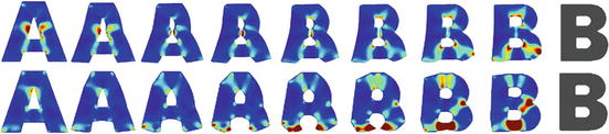
$\displaystyle{ d_{\mbox{ viscous}}(\mathcal{S}_{A},\mathcal{S}_{B}) = \mathbf{L}\left [\left (\mathcal{S}(t)\right )_{t\in [0,1]}\right ]\,. }$

Figure 3 shows two different paths between the same pair of shapes, one of them being a (numerically approximated) geodesic. Note that the chosen dissipation model combines the control of infinitesimal length changes via ${\mathrm{tr}}\left (\epsilon [v]^{2}\right )$ , and the control of compression via ${\mathrm{tr}}\left (\epsilon [v]\right )^{2}$ . Figure 4 evaluates the impact of these two terms on the shapes along a geodesic path.

Fig. 3

A geodesic (top, path length L = 0. 2225 and total dissipation Diss = 0. 0497) and a non-geodesic path (bottom, L = 0. 2886, Diss = 0. 0880) between an A and a B. The intermediate shapes of the bottom row are obtained via linear interpolation between the signed distance functions of the end shapes. The local dissipation rate is color coded as

Fig. 4

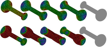
Two geodesic paths between dumbbell shapes varying in the size of the ends. In the top example, the ratio λ∕μ between the dissipation parameters is 0. 01 (leading to rather independent compression and expansion of the ends since the associated change of volume implies relatively low dissipation), and 100 in the bottom row (now mass is actually transported from one end to the other). The underlying texture on the objects is aligned to the transport direction, and the absolute value of the velocity v is color coded as

State-Based, Path-Independent Elastic Setup

Now, objects bounded by a shape contour $\mathcal{S}$ are no longer composed of a viscous fluid but are considered to be elastic solids. To describe object deformations, we aim for an elastic energy which is not restricted to small displacements and which is consistent with the first principles. Alongside the shape space modeling, we will recall some background from elasticity. For details, we refer to the comprehensive introductions in the books by Ciarlet [15] and Marsden and Hughes [47].

For two objects $\mathcal{O}_{A}$ and $\mathcal{O}_{B}$ with shapes $\mathcal{S}_{A} = \partial \mathcal{O}_{A}$ and $\mathcal{S}_{B} = \partial \mathcal{O}_{B}$ , we assume a deformation ϕ to be defined on $\overline{\mathcal{O}}_{A}$ and constrained by the assumption $\phi (\mathcal{S}_{A}) = \mathcal{S}_{B}$ . For practical reasons, one might consider $\mathcal{O}_{A}$ to be embedded in a very soft elastic material occupying $\varOmega \,\setminus \,\mathcal{O}_{A}$ for some computational domain Ω. There is an elastic energy $\mathcal{W}_{\mbox{ deform}}[\phi,\mathcal{O}_{A}]$ associated with the deformation $\phi:\varOmega \rightarrow \mathbb{R}^{d}$ . By definition, elastic means that this energy solely depends on the state and not on the path along which the deformation proceeds in time. More precisely, for so-called hyper-elastic materials, $\mathcal{W}_{\mbox{ deform}}[\phi,\mathcal{O}_{A}]$ is the integral of an energy density W depending solely on the Jacobian $\mathcal{D}\phi$ of the deformation ϕ, i.e.,

$\displaystyle{ \mathcal{W}_{\mbox{ deform}}[\phi,\mathcal{O}_{A}] =\int _{\mathcal{O}_{A}}W(\mathcal{D}\phi )\,{\mathrm{d}}x\,. }$

(4)

This elastic energy is considered as a dissimilarity measure between the shapes $\mathcal{S}_{A}$ and $\mathcal{S}_{B}$ . As a fundamental requirement, one postulates the invariance of the deformation energy with respect to rigid body motions, $\mathcal{W}_{\mbox{ deform}}[Q \circ \phi +b,\mathcal{S}_{A}] = \mathcal{W}_{\mbox{ deform}}[\phi,\mathcal{S}_{A}]$ for any orthogonal matrix Q ∈ SO(d) and translation vector $b \in \mathbb{R}^{d}$ (the axiom of frame indifference in continuum mechanics). From this, one deduces that the energy density only depends on the right Cauchy–Green deformation tensor $\mathcal{D}\phi ^{{\mathrm{T}}}\mathcal{D}\phi$ . Hence, there is a function $\tilde{W}: \mathbb{R}^{d,d}\longrightarrow \mathbb{R}$ such that the energy density W satisfies $W(F) =\tilde{ W}(F^{{\mathrm{T}}}F)$ for all $F \in \mathbb{R}^{d,d}$ . The Cauchy–Green deformation tensor geometrically represents the metric measuring the deformed length in the undeformed reference configuration. For an isotropic material and for d = 3, the energy density W can be further rewritten as a function $\hat{W}(I_{1},I_{2},I_{3})$ solely depending on the principal invariants of the Cauchy–Green tensor, namely, $I_{1} =\mathrm{ tr}(\mathcal{D}\phi ^{{\mathrm{T}}}\mathcal{D}\phi )$ , controlling the local average change of length; $I_{2} =\mathrm{ tr}\left ({\mathrm{cof}}(\mathcal{D}\phi ^{{\mathrm{T}}}\mathcal{D}\phi )\right )$ ( ${\mathrm{cof}}F:=\det F\,F^{-T}$ ), reflecting the local average change of area; and $I_{3} =\det (\mathcal{D}\phi ^{{\mathrm{T}}}\mathcal{D}\phi )$ , which controls the local change of volume. For a detailed discussion, we refer to [15, 78]. We shall furthermore assume that the energy density is polyconvex [18], i.e., a convex function of $\mathcal{D}\phi$ , ${\mathrm{cof}}\mathcal{D}\phi$ , and $\det \mathcal{D}\phi$ , and that isometries, i.e., deformations with $\mathcal{D}\phi ^{{\mathrm{T}}}(x)\mathcal{D}\phi (x) = \nVdash$ , are local minimizers with $W(\mathcal{D}\phi ) =\tilde{ W}(\nVdash ) = 0$ [15]. Typical energy densities in this class are of the form

$\displaystyle{ \hat{W}(I_{1},I_{2},I_{3}) = a_{1}I_{1}^{\frac{p} {2} } + a_{2}I_{2}^{\frac{q} {2} } +\varGamma (I_{3}) }$

(5)

for a ₁, a ₂ > 0 and a convex function $\varGamma: [0,\infty ) \rightarrow \mathbb{R}$ with $\varGamma (I_{3}) \rightarrow \infty$ for $I_{3}\,\rightarrow \,0$ and I ₃ → ∞. In nonlinear elasticity, such material laws have been proposed by Ogden [58], and for $$p = q = 2$$

(the case considered in our computations), we obtain the Mooney–Rivlin model [15]. The built-in penalization of volume shrinkage, i.e., $\hat{W}(I_{1},I_{2},I_{3})\stackrel{I_{3} \rightarrow 0}{\longrightarrow }\infty$ , enables us to control local injectivity (cf. [2]).

Incorporation of such a nonlinear elastic energy allows to describe large deformations with strong material and geometric nonlinearities, which cannot be treated by a linear elastic approach (cf. Hong et al. [36]). Furthermore, it balances in an intrinsic way expansion and collapse of the elastic objects and hence frees us from imposing artificial boundary conditions or constraints.

As in the previous section, the local force per area, induced by the deformation, is described at a point $\phi (x) \in \phi (\mathcal{O})$ by the Cauchy stress tensor σ. It is related to the first Piola–Kirchhoff stress tensor $\sigma ^{\mbox{ ref}} = W_{,F}(\mathcal{D}\phi ):= \frac{\partial W(F)} {\partial F} \vert _{F=\mathcal{D}\phi }$ , which measures the force density in the undeformed reference configuration, by $\sigma ^{\mbox{ ref}} =\sigma \circ \phi \,{\mathrm{cof}}\mathcal{D}\phi$ .

Based on these concepts from nonlinear elasticity, we can now define a dissimilarity measure on shapes

$\displaystyle{ d_{\mbox{ elast}}(\mathcal{S}_{A},\mathcal{S}_{B}):=\min \limits _{\phi,\phi (\mathcal{S}_{A})=\mathcal{S}_{B}}\sqrt{\mathcal{W}_{\mbox{ deform} } [\phi, \mathcal{O}_{A } ]}\,. }$

(6)

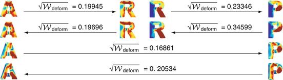
Figure 5 shows some applications of this measure. Obviously, the elastic energy is in general not symmetric so that $d_{\mbox{ elast}}(\mathcal{S}_{A},\mathcal{S}_{B})\neq d_{\mbox{ elast}}(\mathcal{S}_{B},\mathcal{S}_{A})$ . Indeed, by construction, $d_{\mbox{ elast}}(\cdot,\cdot )$ does not impose a metric structure on the space of shapes (we refer to section “Conceptual Differences Between the Path- and State-Based Dissimilarity Measures” for a detailed discussion). Nevertheless, it can be applied to develop physically sound statistical tools for shapes such as shape averaging and a PCA on shapes, as outlined below in section “Elasticity-Based Shape Space.”

Fig. 5

Example of elastic dissimilarities between different shapes. The arrows indicate the direction of the deformation, the color coding represents the local deformation energy density (in the reference as well as the deformed state)

Let us make a brief remark on the mathematical relation between the two different concepts of elasticity and viscous fluids. If we assume the Hessian of the energy density W at the identity to be given by $W_{,FF}(\nVdash )(G,G) =\lambda ({\mathrm{tr}}G)^{2} + \frac{\mu } {2}{\mathrm{tr}}\left ((G + G^{T})^{2}\right )$ (which can be realized in (5) for a particular choice of a ₁, a ₂, and Γ, depending on the exponents p and q), then by the ansatz $\phi (x) = x +\tau v(x)$ and a second-order Taylor expansion, we obtain

$\displaystyle\begin{array}{rcl} W(\mathcal{D}\phi )& =& W(\nVdash ) +\tau W_{,F}(\nVdash )(\mathcal{D}v) + \frac{\tau ^{2}} {2}W_{,FF}(\nVdash )(\mathcal{D}v,\mathcal{D}v) + O(\tau ^{3}) \\ & =& 0 + 0 +\tau ^{2}\left ( \frac{\lambda } {2}({\mathrm{tr}}\mathcal{D}v)^{2} + \frac{\mu } {4}{\mathrm{tr}}\left (\left (\mathcal{D}v + (\mathcal{D}v)^{{\mathrm{T}}}\right )^{2}\right )\right ) + O(\tau ^{3})\,.{}\end{array}$

(7)

In effect, the Hessian of the nonlinear elastic energy leads to the energy density in linearized, isotropic elasticity

$\displaystyle{ W^{\mbox{ lin} }(\mathcal{D}u) = \frac{\lambda } {2}\,\left ({\mathrm{tr}}\epsilon [u]\right )^{2} +\mu \,\mathrm{ tr}\left (\epsilon [u]^{2}\right ) }$

(8)

for displacements u with $\phi (x) = x + u(x)$ . This energy density, acting on displacements u, formally coincides with the local dissipation rate diss[v], acting on velocity fields v, in the viscous flow approach.

Finally, let us deal with the hard constraint $\phi (\mathcal{S}_{A}) = \mathcal{S}_{B}$ , which is often inadequate in applications. Due to local shape fluctuations or noise in the shape acquisition, the shape $\mathcal{S}_{A}$ frequently contains details that are not present in $\mathcal{S}_{B}$ and vice versa. These defects would imply high energies in a strict 1–1 matching approach. Hence, we have to relax the constraint and introduce some penalty functional. Here, we either measure the symmetric difference of the input shapes $\mathcal{S}_{A}$ and the pullback $\phi ^{-1}(\mathcal{S}_{B})$ of the shape $\mathcal{S}_{B}$ given by

$\displaystyle{ \mathcal{F}[\mathcal{S}_{A},\phi,\mathcal{S}_{B}] = \mathcal{H}^{d-1}\left (\mathcal{S}_{ A}\bigtriangleup \phi ^{-1}(\mathcal{S}_{ B})\right )\,, }$

(9)

where $A\bigtriangleup B = A\,\setminus \,B \cup B\,\setminus \,A$ , or alternatively the volume mismatch

$\displaystyle{ \mathcal{F}[\mathcal{S}_{A},\phi,\mathcal{S}_{B}] = {\mathrm{vol}}\left (\mathcal{O}_{A}\bigtriangleup \phi ^{-1}(\mathcal{O}_{ B})\right )\,. }$

(10)

Conceptual Differences Between the Path- and State-Based Dissimilarity Measures

The concept of the state-based, elastic approach to dissimilarity measurement between shapes differs significantly from the path-based viscous flow approach. In the elastic setup, the axiom of elasticity implies that the energy at the deformed configuration $\mathcal{S}_{B} =\phi (\mathcal{S}_{A})$

Only gold members can continue reading. Log In or Register to continue