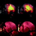
MR for the Investigation of Murine Vasculature

Fig. 1.

MIP view of the renal vessels superimposed with a surface-rendered view of the kidneys for anatomical orientation. The angiogram was reconstructed from a 2D multislice dataset which was acquired from an FOV in sagittal orientation to maximize the inflow effect for the vessels running from the aorta (A) to the kidney. Signals from the portal system of the liver (L) and the chambers of the heart (H) are less marked due to cardiac and respiratory motion.

A more adequate 3D view is obtained from surface or volume-rendered datasets as carried out for visualization of the kidneys within the angiogram in Fig. 1. For both methods, in a first step the user has to define intensity intervals in order to discriminate the background. The spatial impression for a calculated object surface is improved by light effects in the so-called surface-shaded display (SSD) representation. However, surface rendering of an object requires rather extensive work from the user and is therefore superseded by volume-rendering reconstruction. For this technique, the whole image volume is kept in the working memory with intensity or color (RGB) values stored together with opacity information. The main advantage of volume compared to surface rendering is that no interior information is discarded, allowing for viewing and volumetrically quantifying the 3D dataset as a whole. Segmentation of adjacent voxels within the pre-defined intensity interval can easily be performed by defining a seed point via mouse click. However, storing and recalculating of this multidimensional vector is very time consuming and necessitates powerful computers. In Angiotux (see Section 3.6), handling of 3D objects in terms of translation, rotation, and zoom can be accelerated by omitting all vector elements lying outside the defined intensity interval.

3.6 Quantification Methods

Tomographic slices can be analyzed by planimetrical determination of luminal areas using, e.g., the ParaVision (Bruker, Ettlingen, Germany) Region of Interest (ROI) Tool or can be automatically derived by an edge-detection algorithm.

For analysis of the Fourier-transformed 3D MRI datasets, the Angiotux program based on the freely available package Eccet for processing and visualizing voxel data in 3D and 4D can be used (1). With this software vessel segments can be sectioned with a plane freely adjustable in any orientation. An algorithm for the measurement of vessel lengths is implemented in order to account for curvature and varying diameter. Segmented regions are assigned to defined colors and absolute volumes are quantified by counting the voxels of these colors.

Since the intensity in angiographic images is mainly determined by flow velocity which rapidly decreases near the vessel walls due to a laminar flow profile, vessel sizes may be underestimated by 2D or 3D image analysis. Calculation of absolute vessel sizes may further be complicated within longitudinal experimental series of pathological models by alterations in body weight (animal size) or also anesthesia. To account for the latter effects, it is recommended to relate the areas/volumes to a vessel area or segment at the contralateral side that is defined by anatomical landmarks. Using such ratios will cancel out a variety of error sources and greatly reduces the standard deviations of the individual parameters, so that differences between experimental groups can be more sensitively detected.

There are different approaches to determine flow velocities and/or volume flows from gradient echo images (4–6). An alternative and straightforward 2D method is illustrated in Fig. 2a showing a vessel and two slices for saturation and imaging, respectively, positioned perpendicular to flow direction. Excitation of both slices is separated by a fixed time delay (Δt) and a variable gap (g) which can be continuously increased, thereby altering the image intensity as shown in Fig. 2b. If an identical thickness d = d _s= d _mis used, the general intensity progression simplifies to a curve with only one distinct minimum as illustrated in Fig. 2c. This graph shows the signal intensity against the interslice gap for two tubes of diameter D, in which water is flowing with identical velocity but in opposite directions. Both minima nearly coincide at a flow of 2 mL/min as calculated by

$\dot V = \frac{{\pi D^2 \left(g_{\min } + d\right)}}{{4\Delta t}}$

and which was confirmed by direct measurement with an ultrasonic flow meter (Transonic Systems Inc., Ithaca, NY, USA).

To assess alteration in vascular architecture from in vivo measurements, the cross section of the vessel has to be determined, which can automatically be performed by edge-detecting the circumference of the vessel lumen. If the tomographic slice is not exactly perpendicular to the flow direction, the calculated flow velocity has to be corrected (see below). In contrast, volume flow is not significantly affected, since the decrease in v is nearly compensated by an increasing cross section. If d _s≠ d _mis chosen, the equations above can also be used with d replaced by the maximum (for gap g ₂ in Fig. 2b) or the minimum (for g ₃) of both values d _mand d _s.

Generally, positioning of a slice perpendicular to the vessel direction as estimated from the scout images is straightforward. However, in most cases, it is very difficult to realize a true right angle with respect to the third dimension. Assuming a circular vessel cross section, the extent of deviation from the perpendicular position is reflected by the quotient of both radii of the resulting ellipse (Fig. 3a). If the vessel is angled by θ, the length of the semimajor axis is given by r/cos(θ) with the vessel radius r corresponding to the semiminor axis length. To correct cross section, vessel diameter, and flow velocity for θ, an analysis of the elliptical shape should be performed. Figure 3b shows a fit of a polygon describing the circumference of a vessel lumen to a tilted ellipse (see Note 14). The points of the polygon were automatically obtained by edge detection. In this example, the angle θ was calculated from the radii to be 54°.

Fig. 2.

Flow quantification using a saturation and an imaging slice separated by the gap g. (a) Definition of variables with thicknesses d _mand d _sand velocity v. (b) Theoretical curve for the general case d _m≠ d _s. If the interslice gap is continuously varied at fixed Δt between saturation and measurement, significant changes in intensity are expected to occur at the gaps labeled as g ₁ to g ₄ (g ₁ = vΔt − d _s− d _m; g ₂ = vΔt − Max(d _s,d _m); g ₃ = vΔt − Min(d _s,d _m); g ₄ = vΔt). (c) A phantom with two tubes (∅ 500 μm) of identical velocity but different flow directions was used for flow quantification. In both tubes, the intensity minimum was located at a gap attributed to a flow of ∼2 mL/min, identical to the value determined concomitantly by an ultrasonic flow meter.

Fig. 3.

Elliptical correction for cross section and velocity. (a) Slicing the vessel at an angle θ ≠ 0 leads to an elliptical cross section in the image. (b) ROI points defining the luminal border fitted to a tilted ellipse. The parameters of the fit are the coordinates of the center of the ellipse (x ₀ , y ₀), its semi-axes (r _x, r _y), and the tilt angle ϕ (for uniqueness: 0 ≤ ϕ < 90°).

3.7 MRA Applications to Pathophysiological Models

In the following subsections, selected MRA examples are provided representative of the large number of applications in studying the vasculature of mice or small animals in general.

Only gold members can continue reading. Log In or Register to continue