MR Oximetry

where SI_nis the signal intensity at each time point, SI₀ is the initial signal intensity, and TE is the echo time. One needs to keep the units consistent. The same equation holds for ΔR ₂ if one obtains data using a spin echo sequence.

For quantification of multi-echo data, one can fit a single exponential function where:

${\textrm{S}}{{\textrm{I}}_n} = {\textrm{S}}{{\textrm{I}}_0}\ {{\textrm{e}}^{( - {\textrm{TE}}/{\textrm{T}}2)}}$

where SI_nis the signal intensity at a given echo time, TE, and SI₀ is the signal intensity at TE = 0. One can also transform the y-axis into a log function and plot as a semi-logarithmic plot (Fig. 1). The author is not aware of BOLD studies using multiexponential fits, but recognizes that these would be appropriate if the number of echoes is sufficient. Examples of multi-echo analysis of T ₂, which the reader can use as an entry into the issues involved with quantifying multi-echo data, can be found in (20, 21) (see Note 9).

Key variables to control for are systemic oxygenation, motion, and blood flow.

Quantification can be done on a voxel-by-voxel basis or on an ROI basis. The analysis pattern, or workflow, can be undertaken by measuring SI within the ROI and calculating average values or one can undertake the quantification on a voxel-by-voxel basis. After such voxel-based quantification, one can obtain statistical information over the ROI (22).

The changes in SI relate to changes in R ₂ or R ₂*. Both of these parameters change linearly with the deoxyhemoglobin content (3) which, in turn is a reflection of tissue oxygenation (see Note 1) (Fig. 2).

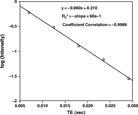
Fig. 1.

A semi-logarithmic plot of SI vs. echo time for quantification of R ₂* in a rat brain. As this is a standard mathematical function for a single exponential decay, if the plot results in a linear fit then one can assume that the decay curve is adequately described by a single exponential function. (Reproduced from (43) with permission from Wiley-Liss Inc.).

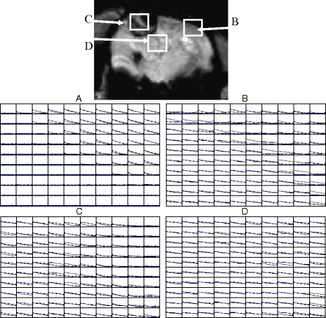
Fig. 2.

An example of voxel-by-voxel processing and the variations in the decay function in vivo. A rat with a glial tumor was studied. A multi-echo gradient echo sequence was used. The upper image shows a cross section of the brain. Below are voxel-by-voxel plots of SI vs. TE. Due to the small size of the voxels in the figure, the axis labels have been omitted. SI is in arbitrary units and the TEs are 9, 15.5, 22, 28.5, and 35 ms. Plot A shows data from the lower left of the head, out of the field of view, that contains noise and muscle. B shows normal brain in the lower left. C is from tumor. D is a second tumor region. There are two lines in each voxel, one while breathing control gasses and the other while breathing hyperoxygenated gas of 95% O₂ and 5% CO₂. The key point to this figure is that, on close examination of voxels, there are clearly voxels that do not show a simple exponential decay function within the tumor. Such deviation from an exponential function is relatively common and care is needed to prevent any misinterpretation that may arise. (Reproduced from (43) with permission from Wiley-Liss Inc.).

3.3 ¹⁹F, T₁ MRI

This method relies on two key points. One is that there is no inherent ¹⁹F signal in living systems under standard conditions and the other is that there are fluorinated hydrocarbons which have a ¹⁹F resonance with a T ₁ relaxation time that is related to the surrounding oxygen concentration.

In these studies, one injects the ¹⁹F tracer and undertakes either ¹⁹F-spectroscopy or MRI. Imaging can also include dual nuclei MRI which, when carefully done to ensure similar RF homogeneity between nuclei, allows the oxygen images to be overlaid on an anatomical ¹H MRI.

Before injection, one should calibrate the relaxation rate R ₁ by undertaking phantom studies. Under controlled conditions, measure the R ₁ vs. oxygen in solution. Oxygen can be measured as pO₂ (mmHg, torr, or kPa), or concentration (% O₂, mM, or ppm). If one is using percentage (i.e., equilibrating with 10% O₂, be sure to control for atmospheric pressure. For instance, 10% O₂ is 75.6 mmHg at sea level but only 67.8 mmHg at 1000 m of altitude (23).

The compounds to be used vary in the number of fluorine nuclei adding to the signal, cost, and availability. The options are listed in Section 2.

Material can be injected intravenously or directly into the tissue. If the data collection is done in a short period after injection, then substantial ¹⁹F signal may arise from the blood after an intravenous injection. It is possible to inject the material and then image hours after injection. This has been done successfully with implanted tumors (10). Under these conditions, the signal may arise from within cells. A confounding issue is that it is not clear which cells contain the ¹⁹F.

It is useful to undertake a pilot study to determine an optimum time for imaging whereby there remains sufficient material in the tissue.

Imaging involves quantification of T ₁. There are many methods available and one needs to assess the fastest and most sensitive method available on the particular scanner (see Note 7).

Prepare the animal for direct injection or intravenous injection. For preparation of an injection of TF-MISO, dissolve in sterile saline solution (5 mg/mL) (11). HFB has been injected undiluted at 3 μl per injection (24).

As most tissues have low pO₂, reduce the pO₂ in the perfluorocarbon by bubbling with N₂ before use (24).

Inject using a small gauge (29G) in multiple tracks to improve penetration.

Position in the MRI, shim, and tune the RF coils.

Undertake localizing MRI using ¹H, T₂w multislice to determine the ROI. This is usually fast, low resolution MRI often with a matrix of 64 × 64 to identify anatomy. A common sequence is a FLASH-type sequence (25) with a relatively low flip angle to reduce T ₁ weighting (40–60°) combined with a short TR to minimize acquisition time (100–300 ms). The field of view and orientation to be used is determined at this stage by optimizing the scout image.

Change to the ¹⁹F frequency and do adjustments like tuning, matching, and flip angle calibration.

A range of sequences may be used. The goal is high sensitivity and rapid acquisition time. Options include snapshot flash inversion recovery (24), a driven equilibrium sequence (13, 26), and EPI-inversion recovery (9).

Quantify T ₁ and compare with pre-determined calibration curves using the same sequence. The equation used to quantify T ₁ depends on the acquisition method. Standard saturation or inversion recovery data are fit to a single exponential recovery curve where MRI signal intensities are plotted against a range of recovery times from either an inversion or saturation pulse (see Note 10). Faster imaging can be done with a range of methods including echo planar and fast low angle imaging (25, 27). State-free precession data are fit to more complex models (28). It is accepted to threshold to remove voxels with random noise (12).

3.4 ¹H, T₁ MRI

Oxygen in solution influences the T ₁ relaxation time of the solution. In living systems, there is a unique opportunity to undertake MRI oximetry within fluids. This has been done in the eye solely by quantifying the T ₁ of the solution within the eye—the vitreous. A method termed the retinal oxygenation response (ROR) was developed whereby changes in T ₁ within the vitreous are monitored during a step function in inspired O₂ (29).

A major potential source of artifact is the blinking response. This can be reduced or eliminated by a paradigm where the subject holds as still as possible for 10–15 s without blinking during which the MRI can be obtained with fast imaging methods. As animals rarely blink during anesthesia, movement is less of a problem with animal studies. One can cover the eyes with ointment to keep the eyes moist and comfortable during the study.

Position subject in the MRI. Subject is instructed to visually target a spot when requested. It is helpful to place gauze over the alternate eye.

Place a face mask for administering breathing gases. It is usually adequate to initiate with room air.

Place a phantom of water near the eye within the field of view. Isolate the phantom from the skin as much as possible to prevent heat transfer from the subject, which would warm the phantom and so alter the T ₁.

Practice a blink/no blink cycle with a human subject before imaging.

Initiate MRI. Obtain a series of baseline T1w images (at least three). One of the simplest methods would be quantifying changes in SI collected using a snapshot FLASH sequence (TR = 22 ms, TE = 7 ms, flip angle 12° at 1.5 T (30); see Note 7).

Change the breathing gas to 100% O₂. Breath the new gas for at least 5 min. The goal is a PaO₂ of greater than 350 mmHg and a PaCO₂ of 35–45 mmHg (29).

Obtain a new localizer image to assist with coregistration of image plane.

Collect hyperoxia images as needed (at least three).

Calculate ΔSI either on an ROI or a voxel-by-voxel basis.

10.

Model against published values of ΔSI vs. pO₂ in saline. A relaxivity of 1.75 × 10⁻⁴ s⁻¹ mmHg⁻¹ has been used (31) and modeling has been undertaken to transform data to mmHg of O₂ (29).

4 Notes

If total hemoglobin is constant, then ΔdeoxyHb will change with the saturation of blood. The link between saturation and pO₂ is non-linear. One needs to be aware of the shape of the oxyhemoglobin dissociation curve if one wants to make comments on pO₂. Many factors influence the magnitude of the ΔR ₂* effect although the result is that ΔR ₂* is linear in brain over a wide range of hemoglobin saturations. Confounding effects such as vessel orientation, Hb content, flow, and red cell geometry will change the ΔR ₂* vs. deoxyHb content relationship (32, 33).

Field sensitivity is important. BOLD methods are more sensitive at higher fields. The balance is that artifacts due to susceptibility are also higher. The R ₂ is relatively more sensitive to microvasculature than R ₂* but has lower sensitivity. When using high fields (7 T or more), it may be desirable to use R ₂ instead of R ₂* as the susceptibility artifacts are less with R ₂ and the sensitivity at high field makes ΔR ₂ quantification possible. For an introduction to the literature on field dependence, see (34, 35). For a discussion on vessel size dependency, see (36–38) (see also Chapter 8).

Only gold members can continue reading. Log In or Register to continue