Volumetry and Other Quantitative Measurements to Assess the Rodent Brain

Fig. 1.

A digital image with a matrix of 6 × 4 (0.06 × 0.06 mm in-plane resolution) and five 0.1 mm thick slices with a 0.05 mm slice gap.

Image registration: Image registration is the process of transforming one image, the source image, in such a way that it can be compared to another image, the target image.

The comparison of the images is done by a similarity measure, which assesses how alike the images are. The transformation of an image can be done either affine or nonlinear: Affine transformation allows only global shifts in location, rotation, and scaling, so the transformation is equal for each point in the image. Nonlinear transformation allows for a different transformation for each voxel in the image. A nonlinear registration might potentially change the shape of the image completely depending on the accuracy of the registration. The result of a nonlinear registration is a deformation field, which is an image with the same dimension as the original image, where each voxel contains a 3D vector indicating the local change of that voxel to go from the source image to the target image. Figure 2 shows an example of a 3D deformation field overlaid, as a result from warping synthetically deformed image (b) (the source), onto its original, image (a) (the target).

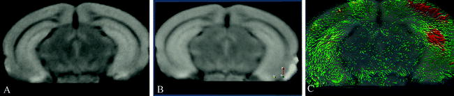
Fig. 2.

An illustration of a nonlinear registration of two time points (a) and (b) and the resulting deformation field (c), which is displayed on top of the warped image b. Each vector indicates to the corresponding voxel in image a. Color coding can be used to indicate the amount of displacement in voxels or in millimeters. The images were acquired in vivo with T ₂-weighted protocol on a Bruker 9.4 T system, with the parameters: TE = 12.76 ms, TR = 4000 ms, RARE factor = 4, FOV = 18 mm², matrix = 200 × 200, thirty 0.25 mm slices, 12 averages.

Image Normalization: Normalization is the process of standardizing images, so that all images have the same orientation, size, and resolution. It places the homologous regions of the several brain images as closely into spatial alignment as possible so that the various brain structures can be compared and analyzed automatically.

The normalization is done by affine or nonlinear registration to a standard reference image. A standard reference image is defined as an average MR image, constructed from brain images of a representative population, which is spatially oriented in a standard viewing direction and has an equal or preferably higher resolution than the group of MR images, which are compared to the reference. The higher resolution of the reference image decreases the effect of partial volume effects in a later stage of the analysis.

A standard reference image should be representative for the population to which it is compared. Therefore, the choice for a standard reference image can be a single mouse brain, or a group average (1). A number of standard mouse brain MRI atlases are freely available (2–4) but as scan parameters and mouse strains vary widely, many people prefer to develop their own reference brain atlases (see Note 1). A good tool to develop in-house mouse reference brains is developed by Mouse BIRN (5). Figure 3 shows an example standard reference image for in vivo and ex vivo MRI.

Fig. 3.

The MRI atlas used for in vivo (e, g) and ex vivo (f, h) MR images with their manual segmentations (a, b, c, and d) and corresponding names and abbreviations. For a better understanding, the abbreviations for the brain structures are in upper case where the abbreviations for brain tracts are in lower case. All images are acquired on a Bruker 9.4 T scanner. For the in vivo images a T ₂-weighted multi-slice spin echo sequence with TR/TE = 6000/35 ms (four averages) was used with a scanning time of 102 min (matrix size of 256 × 256, 40 slices and a resolution of 97.6 × 97.6 × 200 μm³ per voxel). Ex vivo imaging was performed using a T ₁-weighted 3D gradient echo protocol, with TR/TE = 17/7.6 ms, flip angle 25°, and a total scan time of 10 h. The ex vivo volume had a matrix size of 256 × 256 × 256 and an isotropic resolution of 78.1 μm per voxel. (Reproduced from Ref. (6))

Image segmentation: The segmentation of an image is the manual or automated delineation of structures in the image (6, 7). These segmentations can be visualized in 2D or 3D and might used as input for volumetry.

3 Statistics in Quantitative Morphology

Although the choice of a particular statistical test is dependent on the measurements which are performed on the brain, the procedure of a statistical test is similar for all morphometry methods. In this section, we explain the basic principles of statistical testing and how these statistical tests are incorporated in morphometry methods.

Producing and interpreting a p-value: First a null hypothesis and an alternative hypothesis have to be defined. In our experiment, we try to collect as much evidence as possible to prove the null hypothesis is wrong, so we can reject our H₀ and can state that the alternative hypothesis is true with a certain reliability. After the formation of the hypotheses, the experiment is performed, including the measurements on the brain. These measurements are than used as input for a statistical test. The outcome of the test is a p-value, which is an indication of the likelihood that the situation that is observed in the experiment, has occurred by chance. As statistical tests work with chances, there is always a probability margin that an error is made, either H₀ is rejected when it should not be (type 1 error) or H₀ is accepted although this is not true (type 2 error). Therefore, this error margin has to be reported; usually only the type 1 error is reported. Reporting a type 1 error can be done in two ways, either by giving the p-value directly or by thresholding the results at a predefined significance level α. With this significance level, a statement is made about the maximal error that is allowed when rejecting the H₀. In clinical experiments, this level is usually set to 0.01, which indicates that if the same experiment is repeated 100 times, there is on average one case for which the H₀ is rejected falsely.

Multiple-test correction: In most automated quantitative morphometry methods, a certain hypothesis about group difference is tested for each voxel separately, as explained in the methods section. This results in a p-value for each voxel. These p-values are displayed in a so called statistical parametrical map (SPM), which indicates the significant differences per voxel represented by some color scale usually with the significance overlaid on an MR image to indicate the locations of the significant differences. An example of a SPM is given in Fig. 4. All these tests are, unless otherwise specified, independent tests: We need multiple-test correction if we want to draw a general conclusion on the brain instead of the individual voxels (8), i.e., the hypothesis that the brains of the two groups are significantly different instead of a single voxel.

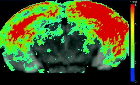
Fig. 4.

A statistical parametric shows a statistical parametrical map (SPM) for uncorrected p-values. The probability scale is overlaid on a MRI image for a better interpretation of the data (unpublished data). The images were acquired in vivo with T ₂ weighted protocol on a Bruker 9.4 T system, with the parameters: TE = 12.760 ms, TR = 4000 ms, RARE factor = 4, FOV = 18 mm², matrix = 200 × 200, thirty 0.25 mm slices, 12 averages.

Multiple-testing refers to the testing of more than one hypothesis at the time, where each test has its own error margin.

For example, two groups of brain MR images from the same population are tested for group difference. The MR images have a 256 × 256 × 128 volume with 8,388,608 voxels. If all hypotheses are tested with α = 0.01, on average, 83,886 incorrect rejections of the H₀ are done and thus 83,886 significant voxels might appear to be different just by chance! If we do not correct for this effect, we might draw the conclusion that the groups from the same populations are significantly different.

Multiple-test correction can be done in several ways, of which the following are advised for multiple-test correction in morphometry (8–10).

Bonferroni correction: This is the most stringent and most straightforward correction. This test is the best method for truly independent voxels; however, as the voxels in the brain are correlated, Bonferroni correction is usually too conservative: it avoids false rejections of H₀, but thereby severely increases the chance of a type 2 error. To correct for multiple test with Bonferroni, H₀ per voxel should be rejected if α/n ≤ 0.01, where n is the number of tests, thus the number of voxels in the volume.

Random field theory: As we should only perform Bonferroni correction on independent voxels, random field theory is used to determine clusters of dependent voxels, so multiple-test correction is only applied on the clusters instead of the voxels. This method requires a smooth SPM, which means that its values change gradually and it has no sharp transitions of probabilities. If a smooth SPM cannot be obtained, the resampling method is advised.

Resampling: The resampling method uses permutation tests to determine the corrected p-values. A permutation test iteratively randomizes the two groups and tests if the original situation is significantly different from the randomized groups (11). In general, this method has a high accuracy—higher than the random field theory. But this method is computationally very expensive and much slower than the Bonferroni and random field theory corrections. Therefore, in practice, it is less applied.

4 Materials

3D MR images of two groups of mice, a test and control group, acquired according to the same protocol and with sufficient quality (see Notes 2, 3, and 4).

A computer with a RAM of minimal 2 GB, preferably 4 GB and CPU power of around 3.0 GHz. (see Note 5).

Image processing software, such as SPM, ImageJ, or Amira (see Note 6).

Statistical software package, such as SPSS, MATLAB, or R (see Note 6).

5 Methods

All quantitative morphometry methods described in this chapter follow the same basic protocol (see Note 7):

Acquire MR images of the two groups of mice.

Find summarizing properties for the structure of interest, the so-called features, which may discriminate between the control group and the test group. Good features might be the volume in mm³, the location of anatomical landmarks, the outer boundary of the structure indicated by landmarks or segmentation (see Note 8).

Use your software package to extract these features for all images in your dataset.

Use your statistical package to test the extracted features to detect a significant difference between the groups.

Based on the results, check the original data if some of the signficiant differences can be explained by any artifacts, misalignments, or misregistrations (see Note 9).

Report your result (see Note 10).

5.1 Manual Volumetry

Volumetry is considered the standard manual approach. This section describes the process of quantification of the brain image by measuring the volume of the structures of interest. The volumetry protocol is based on three steps:

Segmentation: Use the segmentation tool in your image processing package to segment the structure of interest and ask a second expert to check all segmentations (see Note 11).

Volume calculation: Most packages providing segmentation tools also give the volume in mm³ of the segmented structures. If only the number of voxels is given, the volume can be calculated with the following formula: V = N × S = N × (R _x× R _y× R _z), where V is the volume of each segmented structure, N is the number of voxels in the structure. S represents the volume of a single voxel, which can be found by the resolution of the x-, y-, and z-directions (R _x, R _y, and R _z) (see Note 12).

Only gold members can continue reading. Log In or Register to continue