MRI in Animal Models of Psychiatric Disorders

Fig. 1.

Stress hormones and the onset of the stress reaction.

2 Materials

2.1.

Anaesthesia: the animal is usually kept under anaesthesia for the entire MRI experiment to prevent animal discomfort and motion artifacts. We prefer inhalation anaesthetics, as these are easily regulated. Alternatively, for relatively short MRI protocols, injectable anaesthetics may be used.

Isoflurane and isoflurane vaporizer.

Oxygen/air or oxygen/nitrogen carrier gas. This may be bottled or dispensed via a wall outlet. It is advisable to use dedicated flowmeters with a dosage range suitable for small animals (0.1–2 L/min). Some laboratories routinely use nitrous oxide as part of the gas mixture because of the mild analgesic properties; however, be aware that overexposure to nitrous oxide is a severe health risk to the researcher.

Anaesthesia mask and tubing. These may be integrated into the animal bed of the MRI scanner.

Rodent induction box.

Scavenger unit. If you are working in a closed space, it is advisable to scavenge the anaesthetic gasses, e.g. with a carbon filter.

All supplies may be purchased via laboratory or veterinary supply companies (e.g. AgnTho’s AB, VetTech).

2.2.

Monitoring equipment required to assess the physical well-being of the animal:

Device for monitoring respiratory rate, e.g. a pressure-sensitive cushion.

Device for monitoring cardiac activity (optional).

Heating system with rectal temperature probe (or homeothermic pad).

Monitoring device for blood gases (optional).

Monitoring equipment often can be acquired through manufacturers of MRI systems, or alternatively at suppliers of laboratory or veterinary equipment (e.g. SA Instruments, Rapid Biomedical). All devices need to be MRI compatible.

2.3.

Imaging equipment:

An animal MRI system (the most commonly used are the Bruker and Varian systems) with animal cradle and a resonator adjusted to the size of the head, usually about 15 mm diameter for a surface coil and 20–25 mm for a volume coil. For different magnetic field strengths or manufacturers, the protocols described in the Methods section need adjusting. Usually the manufacturer provides a number of standard protocols that are good starting points for your own experiment.

2.4.

Data processing software:

MRI data: ImageJ is free software that allows the manual delineation of the regions of interest within the scans. If the obtained data are not in DICOM format, a plug-in specific for the type of data acquired by your system needs to be installed. The plug-ins are also freely available.

MRS data: The LCModel/LCMgui package produced by Stephen Provencher Inc., is currently the standard software for processing 1D MRS data. Besides the package, the user also needs a library of individual metabolite spectra.

3 Methods

MRI and MRS are techniques that allow in vivo investigation of tissue composition and structure. See Note 3 for a few considerations on their limits. The present section includes a detailed description of basic MRI and MRS techniques performed on mice and rats under isoflurane anaesthesia. The MR protocols depend on the animal model (see Note 4 for a discussion on the choice of animal model). Brief descriptions of several more advanced techniques that can be used in order to acquire more specific data are given in Notes 5–7.

3.1 Data Acquisition

The MRI sequences provided here are based on a vertical 9.4 T Micro-imaging system (Bruker Biospin, Rheinstetten, Germany). ParaVision 5.0 was used for image acquisition. The protocol is suitable for other systems and other manufacturers, but the parameters and routines may have different names; please check the manufacturer’s manuals.

3.1.1 Prepare Scan Protocol

Decide on a scanning protocol, depending on the desired scan (see Fig. 2 for examples).

Use a T2W protocol for a normal anatomic scan (see Table 1)

Use a T1W protocol if using a contrast agent (see Table 2)

Use a FLAIR protocol to acquire more anatomical detail and suppress the bright signal from the ventricles (see Table 3)

Decide on a 3D or 2D geometry, depending on the amount of time available for scanning.

Acquire a 3D scan, if enough time available. This will provide a high resolution image that allows multi-planar delineation of the region of interest, resulting in quite an accurate measure of its volume.

Acquire a multi-slice 2D scan. In this case, the accuracy of the results can be increased by acquiring two data sets in different orientations for each sample: one sagittal and one coronal.

If desired, include an MRS scan. The most commonly used MRS sequence is the point-resolved spectroscopy (PRESS) sequence (see Table 4).

If the standard parameters as given in Tables 2–4 do not satisfy your needs or if you are working at different field strength, you may adjust the parameters (see Note 8 for more details).

Repeat Steps 1–4 if several different scans are desired. Keep the total scan time preferably within 2 h; above 2 h of scanning, consider the effects of dehydration and physiological instability (see Note 9).

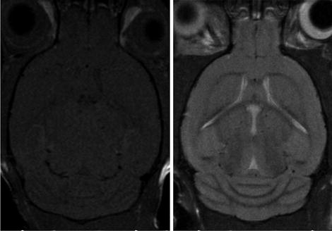
Fig. 2.

MRI images of the mouse brain (axial slices): T1W image (left); T2W image (right).

Table 1

Low- and high-resolution T2W MRI settings for a 9.4 T spectrometer

T2W, 9.4 T	Mice		Rats
Parameters	Low resolution	High resolution	Low resolution	High resolution
Spin echo/TURBO factor	Fast spin echo/8	Fast spin echo/8	Fast spin echo/8	Fast spin echo/8
TE/TEeff/TR (ms)	9/28/4000	9/28/4000	9/28/4000	9/28/4000
Res/FOV (mm²)/matrix	0.100²/25.6²/ 256	0.078²/19.2²/ 256²	0.156²/40²/ 256²	0.089²/35²/ 392²
Slice thickness (mm)/no. of slices	1/10	0.3/20	1/20	0.5/20
Averages/scan time (min)	1/2′8^″	12/25′36^″	1/2′8^″	6/19′36^″

Table 2

Low- and high-resolution T1W MRI settings for a 9.4 T spectrometer

T1W, 9.4 T	Mice		Rats
Parameters	Low resolution	High resolution	Low resolution	High resolution
Spin echo/TURBO factor	Fast spin echo/4	Fast spin echo/4	Fast spin echo/4	Fast spin echo/4
TE/TEeff/TR (ms)	9/9/1300	9/9/1300	9/9/1300	9/9/1300
Res/FOV (mm²)/matrix	0.100²/25.6²/ 256	0.078² /19.2²/ 256²	0.156²/40²/ 256²	0.089²/35²/ 392²
Slice thickness (mm)/no. of slices	1/10	0.3/20	1/20	0.5/20
Averages/scan time (min)	2/2′4^″	12/12′28^″	1/1′2^″	8/12′40^″

Table 3

Low- and high-resolution FLAIR MRI settings for a 9.4 T spectrometer

FLAIR, 9.4 T	Mice		Rats
Parameters	Low resolution	High resolution	Low resolution	High resolution
Spin echo/TURBO factor	FLAIR/4	FLAIR/4	FLAIR/4	FLAIR/4
TE/TEeff/TI/TR (ms)	10/10/825/ 3000	10/10/825/ 3000	10/10/825/ 3000	10/10/825/ 3000
Res/FOV (mm²)/matrix	0.133²/25.6²/ 192²	0.100² /19.2²/ 256²	0.156²/40²/ 256²	0.089²/35²/ 392²
Slice thickness (mm)/no. of slices	1/10	0.5/20	1/20	0.5/20
Averages/scan time (min)	2/4′12^″	8/22′24^″	1/2′24^″	6/22′3^″

3.1.2 Animal Preparation

Decide on the most appropriate time of day for performing the scans. See Note 10 for the interference of the circadian rhythm of rats and mice with the MR measurements.

Bring the animal into the scanning area (see Note 11) and allow habituation for about 60–120 min. Take care in handling and place the animal in an area of mild sensorial to excitation (thus preventing the animal from becoming stressed by bright light, loud noises, strong smells, etc.) (see Notes 12 and 1).

Direct the gas anaesthetics towards the induction chamber.

Turn on oxygen/air mixture at 0.3/0.3 L/min and set the isoflurane to 3.5%.

For alternative anaesthetics, see Note 2.

For measuring on awake animals, see Note 13.

10.

Place the animal inside the induction chamber. Allow 3 min to achieve deep anaesthesia. Depth of anaesthesia can be checked by pinching the paws – no pain reflex should be present.

11.

Redirect the isoflurane flow towards the MRI cradle. Place animal in the cradle in supine position and immediately place the nose of the animal in the isoflurane mask, to prevent awakening.

12.

Turn on the heating system. Insert the rectal temperature probe, if available. Make sure that the animal remains under constant temperature (see Note 14 for implications).

13.

Place the pressure sensitive cushion under the thorax of the animal. Ensure close contact with the animal body (for example by taping a piece of tissue tightly over the back of the animal).

14.

Reduce the isoflurane dosage to 2%. During the entire MR experiment, adjust the isoflurane dose in order to keep the breathing rate at a constant of 50 ± 15 bpm, in order to avoid moving artifacts. Usually the dose gradually decreases to about 1% for a 2 h scanning protocol.

15.

Place the surface coil on the animal’s head, or drag the animal into the volume coil.

16.

Place an external reference tube (2 mM CuSO₄ in H₂O) near the head, inside the coil.

17.

Fixate the head of the animal. Most animal beds have a tooth bar to hook behind the front teeth. Some animal beds have ear bars to prevent head motion. These should be inserted carefully to avoid rupturing the ear drums. A more animal-friendly method is to fixate the head and the coil with memory foam (e.g. standard noise-reducing ear plugs).

18.

If your model requires the administration of certain drugs or contrast agents by i.v. injection immediately prior to the scanning, administer the i.v. injection now.

19.

Place the cradle in the centre of the magnet and connect the coil to the system.

3.1.3 MRI

20.

Create a new scan protocol (“new patient”).

21.

Load a pilot scan #1 provided by your system (“Pilot_GE” for a Bruker system) and tune the coil to resonance (“wobble”).

22.

Run the pilot scan to check the position of the brain in the centre of the coil: 2D gradient echo with TR = 100 ms, TE = 4 ms, one average, rf excitation = sinc7H; 1 ms; FA = 15°, three orthogonal slices of 1 mm with FOV = 30 × 30 mm, matrix 128 × 128, scan time 13 s. When you run scans using automatic acquisitions (“traffic light”), shimming, pulse calibration, and receiver gain adjustment will be done automatically.

23.

Run a second pilot scan and edit the geometry based on the first scout scan. Aim to place three perpendicular fields that intersect on the median lines of the brain.

24.

If necessary, repeat Step 23 after re-editing the geometry based on each previous scout scan, until the positioning on the median lines is acquired.

25.

Open the predefined MRI protocols as determined in Steps 1–5, adjust the geometry based on the last acquired pilot scan, and run the required protocols. If no MRS scans will be performed at this point, continue with Step 32.

3.1.4 MRS

26.

Open the PRESS protocol without water suppression, define the voxel geometry and place it such that the centre of the voxel coincides with the centre of the area of interest.

27.

Ensure that the voxel homogeneity is optimal, using localized shim protocols. Bruker has several options:

Run “method-specific adjustment” of the field homogeneity for the PRESS protocol. Ensure that the voxel is placed in the correct area. Consult the manufacturer’s manual for more details.

Run a Fastmap protocol according to the manufacturer’s instructions.

Run a Fieldmap protocol according to manufacturer’s instructions.

Some tips can be found in Note 15.

28.

Record a water spectrum (water suppression off) with the same TE and TR as the PRESS protocol. Only one average is needed.

29.

Determine the line width of the water peak at full-width-half-height (FWHH). At a Bruker system you can use the macro “CalcLinewidth” to do this automatically. FWHH should be below 30 Hz at 9.4 T. With proper shimming, line widths of about 15 Hz can be obtained in homogeneous brain areas. If necessary, repeat Steps 26–28.

30.

Open the PRESS sequence and run it on the same voxel, with the water suppression and the outer volume suppression ON, according to your imaging system. An example of a ¹H MRS spectrum at 9.4 T has been acquired by Tkac et al. (44) in the mouse brain (see Fig. 3 and Table 5). Note that this spectrum was acquired using a very sophisticated shim set-up and you will usually obtain results that have broader lineshapes.

Fig. 3.

In vivo ¹H NMR spectrum of the mouse brain (C57BL/6) with the volumes of interest (VOIs) centred in the cerebral cortex. Ins, myo-inositol; PCr, phosphocreatine; Cr, creatine; Gln, glutamine; Glu, glutamate; Tau, taurine; Cho, choline; Asp, aspartate; NAA, N-acetyl-aspartate; GABA, gamma-aminobutyric acid; Ala, alanine; Lac, lactate; VOI, volume of the voxel; NT, number of averages. Reproduced with permission from Ref. (82).

Table 4

¹H MRS settings for a 9.4 T spectrometer

¹H MRS, 9.4 T	Mice	Rats
Sequence	PRESS	PRESS
TE/TR (ms)	15/3500	15/3500
No. of points	2048	2048
No. of averages	512	256
Voxel size (μL)^a	10	20
Scan time (min)	30	15

^aGiven for orientation purposes, it depends strictly on the region of interest.

Table 5

Most common brain metabolites involved in psychiatric disorders and detectable in mice and rats

Neuro-chemical compound	Peak position (ppm)	Biological interpretation
NAA	2.02	Neuronal marker, the decrease may reflect neuronal loss, decreased neuronal viability, impaired neuronal function
GABA	2.3	Inhibitory neurotransmitter
Glutamate	2.3	Neurotransmitter, high levels may reflect neuronal damage as effect of anoxia or brain injury, may indicate dopaminergic dysfunction
Glutamine	2.3	Amino acid, serves as substrate for glutamate in the glutamate–glutamine cycle
Myo-inositol	3.56	Sugar, involved in neuronal signalling systems; neuronal marker and astrocyte marker, involved in cell membrane metabolism and osmoregulation
Choline	3.23	Neuronal constituent, sometimes used as reference for quantifying other peaks, may be involved in modulating synaptic activity, was linked with membrane turnover and biosynthesis of membrane-bound phosphatidylcholine
Creatine/ phosphocreatine	3.02	Brain metabolite considered stable, presently used as internal standard

3.1.5 Recovery After MRI

31.

Remove the animal from the magnet and allow recovery in a well-ventilated dark warm chamber, e.g. by placing a heating lamp above the cage.

32.

Check for signs of recovery (the pedal reflex should be noticeable after 1 min).

33.

Check for signs of activity (the animal should be completely recovered within 15 min). Avoid transport to the facility before the animal is completely recovered.

3.2 MRI Data Processing

3.2.1 Manual Delineation and Classification of Images

The experienced observer who will delineate the areas of interest should be blinded to the experimental set-up, in order to avoid bias. Rename the measurement files if necessary.

Load an individual scan into the analysis software of choice. A commonly used package is the free-ware image processing package ImageJ (http://rsbweb.nih.gov/ij/).

Find a slice that can be associated with most certainty with its correspondent histological section in a mouse brain atlas (e.g. http://www.mbl.org);

Open the ROI Manager.

Draw the contour of the region of interest in the particular slice, using the histology atlas as a reference guide.

If the contour is sufficiently precise, save the region of interest in the ROI Manager.

Proceed to the next slice and repeat Steps 5–6.

When all areas of interest have been delimited, the collection of ROIs can be saved.

Calculate the area of delimited regions using the “Measure” function in the ROI manager. It will produce a table that can be copied to an Excel file. For quantitative volume measurements, you need to multiply the number of voxels with the voxel volume, which is (in-plane resolution)² × slice thickness (including slice gap).

10.

The table produced by ImageJ contains also the average intensity of the delineated regions; to assess signal intensity changes, this average intensity should be normalized by an internal or external reference. The reference tube can be used as an external reference. If this is not available, an area of tissue that is assumed to remain constant can be used, such as muscle.

11.

More details on image processing and volumetry can be found in Chapter 15.

3.2.2 MRS Data Processing

Load an individual scan into the LCMgui.

Load the water peak corresponding to the same MRS scan.

LCModel will open a window in which attenuation factors can be provided. These can be calculated from the T ₁ and T ₂ decay times of the water in the region of interest, in order to have the correct estimation of the metabolites concentrations. A formula for the calculation can be found in the LCModel manual (http://s-provencher.com/pub/LCModel/manual/manual.pdf). T ₁, T ₂, and proton density values have to be obtained experimentally, or literature values can be used.

Run the processing.

The output will contain concentrations of metabolites accompanied by the Cramer–Rao lower bound as an estimate of variance. Commonly, a threshold of 20% is used to discard fits with insufficient accuracy and therefore of the estimated concentration.

Only gold members can continue reading. Log In or Register to continue