Object Detection Using Color Features for Colonoscopy Quality Measurements

Fig. 1

Sample frames of (a) Green Bite-block, (b) Blood, (c) Stool areas marked with blue lines, and (d) Normal colonoscopy frame

Typically, upper endoscopy and colonoscopy procedures are performed in the same room at different times. It is necessary to distinguish the type of a procedure prior to execution of any quality measurement method to evaluate the procedure. For instance, stool detection generates useful information only for colonoscopy, but not for upper endoscopy. We need to develop a method to detect the procedure type at the beginning of the procedure so that only colonoscopy-related modules run on the procedure. In upper endoscopy, a bite-block (see Fig. 1a) is inserted for patient protection. By detecting a bite-block appearance, we can distinguish colonoscopy from upper endoscopy
Blood detection plays several important roles in various endoscopies, for example, blood detection in wireless capsule endoscopy (WCE) aims to find abnormal regions in the small bowel. On the other hand, blood detection in colonoscopy has two applications: detection of bleeding and erythema and estimation of whether polypectomies [1] are performed during the procedure. We propose a method to detect blood regions in colonoscopy videos
The diagnostic accuracy of colonoscopy depends on the quality of bowel preparation [10]. Without adequate bowel preparation, missed lesions may be covered by stool. The quality of bowel cleansing is generally assessed by the quantity of solid or liquid stool in the lumen. Despite a large body of published data on methods that could optimize cleansing, a substantial level of inadequate cleansing occurs in 10–75 % of patients in randomized controlled trials [11]. Poor bowel preparation has been associated with patient characteristics, such as inpatient status, history of constipation, use of antidepressants, and noncompliance with cleansing instructions. To assess the quality of bowel preparation, we propose a method to compute the amount of mucosa covered by stool

Since all these objects do not pose any other distinguishable characteristics (i.e., shape or texture) other than color, we use color feature. In our previous work [12], we developed a method detecting stool regions in colonoscopy frames. This method was developed solely for post-processing quality measurement. Consequently, it does not meet the real-time requirement for the real-time quality measurement system. In this proposed study, we extend the previous method to detect regions of bite-blocks and blood with good accuracy in addition to stool and to reduce detection time to satisfy the real-time requirement. The main idea is to partition very large positive examples (pixel values) of each object into a number of groups, in which each group is called “positive plane.” Each positive plane is modeled as a separate entity for that group of positive examples. Our previous method for modeling each plane is very time-consuming. As a result, it does not meet the real-time requirement. To overcome this drawback, we propose to use a “convex hull” to represent a positive plane. The convex hull representation enables real-time object detection. Our experimental results show that the proposed method is more accurate, faster, and more robust.

The rest of the paper is organized as follows. Section “Related Work” discusses the related work. Section “Proposed Methodology” describes the proposed methodology and the three applications for detecting stool, bite-block, and blood. Section “Experimental Method and Results” shows our experimental results. Finally, Section “Conclusion and Future Work” summarizes our concluding remarks.

Related Work

Color-based classification plays a major role in the field of medical image analysis. A significant number of studies on object detection based on color features can be found in the literature. Some of them are briefly summarized in this section.

In [13], we proposed a method to classify stool images in colonoscopy videos using a Support Vector Machine (SVM) classifier. The colonoscopy video frame is down-sampled into equal-sized blocks in order to reduce the size of the feature vector. Some pixel-based values such as average color and a color-histogram of each block are used to form a feature vector for the SVM classifier. Then, a stool mask is made for each video frame using the trained SVM classifier, and some post-processing methods are applied to improve the detection accuracy. The post-processing methods include a majority filter and a morphological opening filter. Finally, the frames having more than 5 % of stool area (pixels) are classified as stool frames. A disadvantage of this SVM-based method is the detection time, which is not fast enough to be used in the real-time environment.

In our previous method [12], we proposed a method to detect stool regions for post-processing quality measurement. First, we partition the data (stool pixel values) set into a number of groups, and model each group as a separate data set. The separate data set is called “positive plane.” For the modeling of each positive plane, it is divided into a number of blocks using a thresholding mechanism. The block division including the number of blocks significantly affects the detection time. Hence, we need to find a replacement of the block division to meet the real-time requirements.

Most related works on blood detection are conducted on wireless capsule endoscopy (WCE) videos. In [14], a methodology was proposed aiming at the detection of bleeding patterns in WCE videos. In this study, the features used are the histograms of hue, saturation, and value [15], and co-occurrence matrix of the dominant colors. These features are then used with a SVM ensemble to detect bleeding patterns in WCE videos. Another method to detect bleeding and other blood-based abnormalities in WCE images was presented in [16]. This work was based on a previously published method in [17]. The segmentation is carried out on smoothed and de-correlated RGB (Red, Green, and Blue) color channels using a fuzzy segmentation algorithm. The segmentation result is then transformed to a Local Global graph, which mathematically describes the local and global relationships between the segmented regions in terms of a graph. This graph is used for merging similar segmented regions. In [18], the detection of bleeding patterns is done in two steps. First, the detection of frames with potential bleeding areas is performed based on the assumption that blocks representing bleeding areas are more saturated than the others. Pre-classification detects a frame as a bleeding frame if at least one block represents a bleeding area. In the second step, the initial classification is verified and refined based on pixel-based multi-thresholding of the saturation and intensity. Finally, a bleeding level is assigned to that particular frame based on the pixel values. The work in [19] uses a Neural Network classifier with chromaticity moments for the classification of bleeding and ulcer regions. All the blood detection methods mentioned above suffer from very slow detection time. Thus, they are not applicable to our real-time environment. To the best of our knowledge, there is no methodology for the detection of a bite-block appearance in the literature.

Proposed Methodology

This section explains the proposed method in detail. The method consists of three stages: Training (Section “Training Stage”), Modeling (Section “Convex Hull Models of Green Bite-Block, Blood, and Stool”), and Detecting (Section “Detecting Stage”).

Training Stage

It consists of eight steps as shown in Fig. 2. They are described in the following subsections.

Fig. 2

Steps in training stage

Training Dataset Generation

In this subsection, we explain Steps 1, 2, and 3 in the training stage (Fig. 2). The domain expert marked and annotated the contents of colonoscopy frames into four classes: bite-block, blood, stool, and normal frames. They are used as training data. Figure 1 shows some sample frames of the four classes used in this study. We extract and store the pixels values from these marked and annotated areas. These pixels contain some duplicate values, which are removed to create a unique set of training examples (pixel values) in RGB color space. As per the property of high discriminative power [20], we transform these pixels in RGB color space into those in HSV (Hue, Saturation and Value) color space.

HSV Conversion

This subsection explains Step 4 in the training stage (Fig. 2). RGB color space is defined by the three chromaticities of the red, green, and blue and represented as a three-dimensional Cartesian coordinate system. RGB is a device-dependent color model. That is, different devices produce given RGB values differently. Thus, an RGB value does not define the same colors across different devices [20]. Also, RGB color channels are strongly correlated. This characteristic makes the RGB color space less discriminative.

HSV color space describes colors in terms of their color (Hue), shade (Saturation), and brightness (Value) [20]. Hue is typically expressed as an angle value from 0 to 360^° representing hues of various colors. In this study, Hue is expressed as a number from 0 to 1 instead of an angle from 0^° to 360^° as seen in (1). Saturation is an amount of grayness in a color and represented as a number in the range of 0 and 1. Value (brightness or intensity) of a color is represented as a number from 0 to 255. In the proposed method, RGB color values of a pixel are converted to HSV values of the same pixel using (1).

$$$ \begin{array}{ccc}H=\left\{\begin{array}{l}\left(\frac{G-B}{\Delta}\right),{C}_{\max }=R\\ {}\left(\frac{B-R}{\Delta}\right),{C}_{\max }=G\\ {}\left(\frac{R-G}{\Delta}\right),{C}_{\max }=B\end{array}\right.& \kern1em S=\left\{\begin{array}{l}0,\kern1.24em \Delta =0\\ {}\frac{\varDelta }{C_{\max }},\Delta <>0\end{array}\right.& \kern1em V={C}_{\max}\hfill \end{array} $$” src=”/wp-content/uploads/2016/03/A303895_1_En_14_Chapter_Equ1.gif”></DIV></DIV><br /> <DIV class=EquationNumber>(1)</DIV></DIV>where <SPAN class=EmphasisTypeItalic>C</SPAN> <SUB>max</SUB> = max(<SPAN class=EmphasisTypeItalic>R</SPAN>,<SPAN class=EmphasisTypeItalic>G</SPAN>,<SPAN class=EmphasisTypeItalic>B</SPAN>), <SPAN class=EmphasisTypeItalic>C</SPAN> <SUB>min</SUB> = min(<SPAN class=EmphasisTypeItalic>R</SPAN>,<SPAN class=EmphasisTypeItalic>G</SPAN>,<SPAN class=EmphasisTypeItalic>B</SPAN>), and Δ = <SPAN class=EmphasisTypeItalic>C</SPAN> <SUB>max</SUB> − <SPAN class=EmphasisTypeItalic>C</SPAN> <SUB>min</SUB>.</DIV></DIV><br /> <DIV id=Sec7 class=$

Positive Plane Generation

This subsection explains Step 5 in the training stage (Fig. 2). Now we have the positive examples of the three object classes (bite-block, blood, and stool) in HSV color space. We project all these examples into HSV color cube in which each channel (H, S, and V) is represented as an axis in the 3D Cartesian coordinate system. This step is illustrated in Fig. 3 in which HSV color cube is shown in the XYZ coordinate system. Z-values are in a different range than the X and Y values, but the same scales are used for illustration purpose.

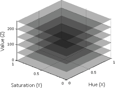
Fig. 3

Placement of planes along value axis

In the next step, we create 256 planes in the HSV color cube along Value (Z) axis so that each integer location of Value axis has a plane parallel to HS planes as seen in Fig. 3. Only a small number of positive planes are shown in the figure. Either H or S axis can be selected as the index axis. Based on our experiments, usage of Value axis as the index axis offers the best detection accuracy. Then, we assign a number (from 0 to 255) to each plane (i.e., Plane#0, Plane#1 … Plane#255). Some planes contain a very small number of positive class examples. Among these 256 planes, hence, we keep the planes in which its positive class examples are greater than or equal to a certain threshold. In our study, we use three for the threshold value which was decided experimentally. Each selected plane is called a “Positive Plane.” Each positive plane contains a subset of positive examples (pixels) and is later modeled as a 2D classifier. For instance, Plane#0 (at V = 0) is treated as a classifier for positive class examples on Plane#0.

Computation of a Convex Hull for Each Positive Plane

This subsection explains Step 6 in the training stage (Fig. 2). For each positive plane selected in Section “Positive Plane Generation”, we generate a convex hull. Algebraically, a convex hull of a dataset X can be characterized as the set of all of the convex combinations of finite subsets of points from X: that is a set of points in the form of ${\sum}_{j=1}^n{\propto}_i{x}_j$ , where n is an arbitrary nonzero positive integer, the numbers, ∝ _i, are nonnegative and sum to 1, and the point x _jis in X. So, the convex hull, H _convex(X) of set X is given in (2), where ∝ _iis a fraction between 0 and 1 in $\mathbb{R}$ (real numbers). The maximum value of k can be the number of data points in the dataset, which contribute to the convex hull.

${H}_{\mathrm{convex}}(X)=\left\{{\displaystyle \sum}_{i=1}^k{\propto}_i{x}_i\Big|{x}_i\in X,{\propto}_i\in \mathbb{R},{\propto}_i\ge 0,{\displaystyle \sum}_{i=1}^k{\propto}_i=1,k=1,2,\dots \right\}$

(2)

To generate a convex hull that adheres to the constraints given in (2), we use the quick hull algorithm introduced in [21]. The basic steps of the quick hull algorithm are given below, and its graphical representation is given in Fig. 4.

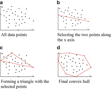
Fig. 4

Convex hull generation using the quick hull algorithm

Find the furthest and closest points from the origin along the x-axis; these two points will be the vertices of the convex hull. Partition the points into two halves using the line drawn between the two points selected (Fig. 4b)

Select a point from one side of the line drawn in Step 1, which is the furthest point from the line. This point along with the two points selected in the above step creates a triangle. The points lying inside of that triangle will be discarded since they cannot be any vertices of the convex hull (Fig. 4c)

Repeat Step 2 for the other side of the line drawn in Step 1

Repeat Steps 2 and 3 on the two new lines formed by the triangle

Iterate until no more points are left

Iterative Outlier Removal

This subsection explains Steps 7 and 8 in the training stage (Fig. 2). After obtaining the convex hull as described in Section “Computation of a Convex Hull for each Positive Plane”, we perform a procedure for outlier removal, in which we remove outliers in several stages in order to improve the overall accuracy of the proposed method. For the outlier removal we use (3). The reason why we are using this equation instead of a typical outlier removal method like “Box plot” is that it is easy to be applied to our convex hulls. Using (3), we remove convex hull vertices from the original data points and recalculate convex hull on reduced data points. The subscript i in the equation represents the number of iterations, which is determined experimentally (i.e., in our study, i = 1) and provided in the beginning of the outlier removal procedure. Outlier removal procedure stops when it iterates i time(s).

${H}_{\mathrm{Convex}(i)}(X)={H}_{\mathrm{Convex}}\left(X-{\displaystyle \sum_{n=0}^{i-1}{H}_{\mathrm{convex}(n)}(X)}\right)$

(3)

As mentioned in Section “Positive Plane Generation”, a positive plane has at least three vertices (positive examples), so this outlier removal is applied to a convex hull with four or more vertices. After performing the outlier removal, we store the positive plane number along with the coordinate values of convex hull vertices for that particular positive plane. This procedure is done for all the positive planes. We then combine all the positive convex hulls in a model. We call this “convex hull model.” This convex hull model is used for the detecting stage.

Convex Hull Models of Green bite-block, Blood, and Stool

In this section, we present three different applications of the proposed method. We use the algorithm mentioned in Section “Training Stage” to generate convex hull models for three different classes of objects: green bite-block, blood, and stool. Although a bite-block could be of any color, the most commonly used bite-blocks in our data set are green. Thus, we design our method to detect green bite-blocks. However, our method can be easily extended to detect a different bite-block color. The selection of positive planes is depicted in Figs. 5a and 6b for each object class. For ease of illustration, we only present a small number of positive planes in this figure.

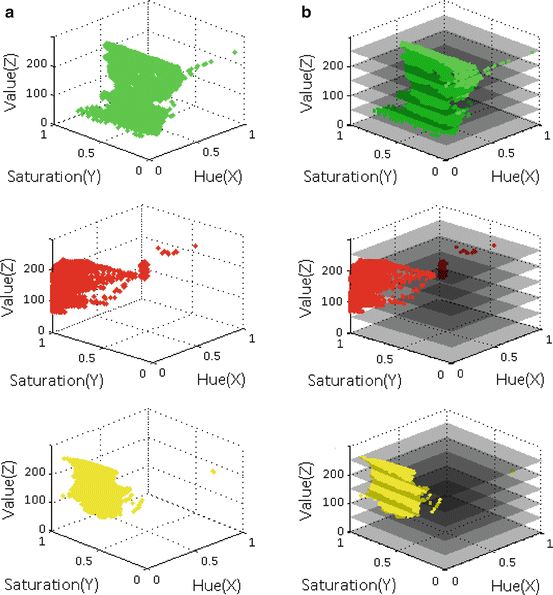
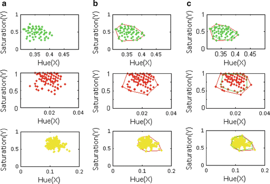
Fig. 5

Selection of positive planes. (a) HSV cubes and corresponding locations of positive example pixels, and (b) Several planes inserted into the HSV cube of (a). First row: Green bite-block, second row: Blood, and third row: Stool

Fig. 6

Examples of convex hulls. (a) Positive class examples projected on a positive plane (plane #200) as looking into the HSV cube in Fig. 5(b) from top. (b) Convex hull (red polygon) for the positive plane and (c) Convex hull (green polygon) after first level outlier removal. First row: Green bite-block, second row: Blood, and third row: Stool

Only gold members can continue reading. Log In or Register to continue