Phase Velocity Mapping
Mark Doyle
PHASE INFORMATION
In phase velocity mapping, the velocity of spins in each voxel is represented in the phase of the spin system. In most instances, the images that we see contain only magnitude information, in that they only represent the magnitude of the spin system. However, each spin is a vector, and can be described in terms of the following two unique quantities:
Magnitude
Phase
Typically, there is no requirement to be sensitive to phase information, and images are reconstructed in such a manner that the phase of the signal does not affect image appearance. Consider the net magnetization vector (M0) that describes the spin system, possessing both magnitude and phase (see Fig. 30-1). When encoding k-space data, the phase of the M0 vector is affected by the applied gradients in a controlled manner, and we note the following two features:
The central point of k-space corresponds to the signal acquired without application of any gradients, that is, all spins are in phase with each other at this single point.
The “phase” of the corresponding image reflects the phase conditions pertaining when the central point is acquired.
PHASE BASICS
The possible range of phase information is as follows:
0 to 360 degrees
0 to 2π radians
Values of phase >2π, or <0, are not uniquely represented and are therefore aliased into the range 0 to 2π radians. Ideally, the phase image should be flat, and have the value of zero for all pixels. However, k-space data are rarely this perfect due to a number of sources, including the following:
Nonidealized gradients
Time dependent eddy currents
B0 field inhomogeneities
Therefore, the “phase information” rarely forms the flat, featureless, image that we might expect (see Fig. 30-2). Distortions of the phase information are typically a function of nonideal phase increments between k-space lines, and between points along the frequency encoding direction.
EDDY CURRENT COMPENSATION
The most disruptive features affecting phase information are time-dependent eddy currents. With each
gradient transition, there is an associated eddy current, which is a current induced in the magnet superstructure (see Fig. 30-3). Eddy currents are transitory electrical currents that oppose the field that generated them. Self-shielded gradients are employed to reduce eddy currents, but these are only partially effective. Eddy current compensation is an additional approach that adds a time-dependant counter current to the gradient waveform, and is applied at each gradient transition point. However, even when employing eddy current compensation and shielded gradients, phase information remains disrupted.
gradient transition, there is an associated eddy current, which is a current induced in the magnet superstructure (see Fig. 30-3). Eddy currents are transitory electrical currents that oppose the field that generated them. Self-shielded gradients are employed to reduce eddy currents, but these are only partially effective. Eddy current compensation is an additional approach that adds a time-dependant counter current to the gradient waveform, and is applied at each gradient transition point. However, even when employing eddy current compensation and shielded gradients, phase information remains disrupted.
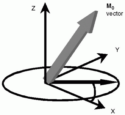 FIGURE 30-1 The net magnetization vector, M0, possesses both magnitude and phase information. Although the phase information of the spin is integral to the k-space encoding mechanism, the phase information is rarely represented in the final image, which is dominated by the magnitude data. |
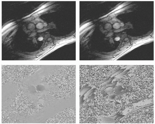 FIGURE 30-2 The left panel shows an idealized magnitude image (top) and phase image (lower). In the phase image, velocity is represented as bright and dark information. The right panel shows corresponding magnitude (top) and phase (lower) images where the phase information is disrupted. This is more typical of the phase that is normally achieved. Notice that the magnitude image is not appreciably influenced by the phase information. |
REFERENCE PHASE IMAGE
It can be appreciated that any process that requires sensitivity to phase information must be able to accommodate the nonideal phase variations present. One way to accomplish this is to obtain a reference image (with nonideal phase variations) and use this to correct the phase encoded image. Therefore, phase subtraction of the reference and encoded images can be used to undo the effects of phase variations, effectively allowing a flat baseline for the phase information to be obtained.
MOVING SPINS AND PHASE
Consider a static spin. Application of a positive gradient followed by a negative gradient forms a gradient echo. The echo peak is the point where all spins (less T2 effects) are in phase with each other. In contrast, a spin moving along the direction of the applied gradients (positive and negative components) will not come back into phase at the echo peak due to the change of position that occurs while the gradients are applied (see Fig. 30-4). Therefore, it can be appreciated that static and moving spins can be differentiated from each other by the phase conditions present at the echo peak. It is possible to design gradient waveforms to control this phase difference such that the difference is linearly proportional to velocity.
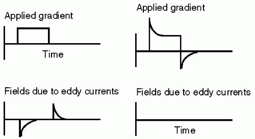 FIGURE 30-3 The left panel shows an applied gradient (top), and the corresponding induced eddy currents (lower panel). Notice that the induced eddy currents are initiated when the main gradient is switched on or off, and that the direction of each eddy currents is dependent on whether the gradient is switched on (negative) or off (positive). The right panel shows the principle of eddy current compensation. In this instance, the waveform of the applied gradient (top) is deliberately distorted to counteract the eddy currents. Following this procedure no, or dramatically reduced, eddy currents are generated. |
BIPOLAR GRADIENTS
In a bipolar gradient, equal areas of the positive and negative gradients are applied. When a bipolar gradient is applied:
Static spins undergo a net zero phase evolution.
Moving spins undergo a nonzero phase evolution.
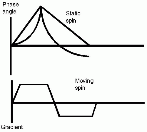 FIGURE 30-4 The spin phase accumulation for a static and moving spin is shown in response to a bipolar gradient
Get Clinical Tree app for offline access
Related posts:Stay updated, free articles. Join our Telegram channel
Full access? Get Clinical Tree


|