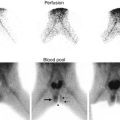
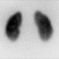
Fig. 4.1
(a–d) Magnetic resonance imaging (MRI) showing renal scars in a 3-year-old girl with reflux nephropathy. Dimercaptosuccinic acid (DMSA) radionuclide scan comparative coronal levels (1, 2) are shown [37]
Basics of Magnetic Resonance Imaging
Phenomenon of Nuclear Magnetic Resonance (NMR)
MRI and nuclear magnetic resonance spectroscopy (NMRS) are based on the phenomenon of nuclear magnetic resonance. All atoms with an odd number of protons and/or odd number of neutrons possess nuclear spin angular momentum and exhibit the phenomenon of magnetic resonance. There are many such nuclei in the body – 1H, 13C, 31P – that exhibit this property, but we will restrict ourselves to the most abundant, i.e., the 1H or proton, as it produces the largest signal and is most commonly used in clinical MRI. This section provides a brief introduction to the basics of NMR and MRI. For a more detailed coverage of the two areas, the reader is referred to books by Slichter and Nishimura [3, 4].
A proton can be thought of as a charged sphere spinning about its axis, which produces a magnetic field. These protons are most commonly referred to as spins in MRI. In the absence of any external magnetic field, the spins are randomly oriented in all directions, resulting in no net macroscopic magnetic field. When placed in a constant external magnetic field B 0, the spins align themselves parallel or antiparallel to B 0. There is a slight excess of spins aligned parallel to the B 0 field, resulting in a net magnetic moment M along B 0. This phenomenon is called polarization. Spins exhibit another phenomenon called precession. While spinning about their own axis, they also wobble around the B 0 field, analogous to the wobbling motion of a spinning top in a gravitational field. This precession frequency is called the Larmor frequency which is the product of the external magnetic field B 0 and the gyromagnetic ratio γ, a constant for each nucleus. At 1.5 T, the Larmor frequency for protons is 63 MHz. Physically, this corresponds to a two-state split in energy levels when spins are placed in a magnetic field, with the energy difference between the states given by the Larmor frequency. When spins make transitions between the two energy levels, it results in absorption or emission of electromagnetic energy (photons) at the Larmor (resonance) frequency. This phenomenon is called nuclear magnetic resonance (NMR).
NMR was first observed and described independently by Felix Bloch and Edward Purcell in 1946. It was soon used in chemistry to interrogate the structures of molecules and study other physical properties such as diffusion, but it was not until 1973 did Lauterbur make the first images by using principles of magnetic resonance in conjunction with linear gradients [5].
Signal Generation
The static B 0 field alone will not produce any useful measurable signal, as the system is in equilibrium. The net magnetic moment M has to be perturbed in order to observe it. This is done by the application of another radiofrequency (RF) magnetic field B 1 for a brief time interval τ and orthogonal to the static magnetic field B 0, which essentially transfers energy to the spins to cross the energy barrier between the two levels. The applied magnetic field is also at the Larmor frequency to elicit the resonance phenomenon. Physically, this can be thought of as applying a torque on M, which rotates it into a different plane, while M continues to precess about the resultant field. The angle θ by which M is rotated is called the flip angle in MRI. The magnetic moment M is usually rotated into the transverse plane orthogonal to the longitudinal B 0 field (i.e., 90° flip angle) to produce the largest signal. The orthogonal RF field B 1 is typically on the order of a fraction of a Gauss compared to the main magnetic field B 0 which ranges from 0.5 to 3 T for most whole-body human imaging systems. After a brief application of the RF field B 1, the net moment M, now in the transverse plane (x-y), continues to precess about B 0 and, by Faraday’s laws of electromagnetic induction, induces a signal voltage in a coil placed in the transverse plane. In NMR spectroscopy and the early days of MRI, the RF coil used to produce the B 1 RF field was also used to receive this induced voltage signal, which is also at the Larmor frequency. In modern whole-body MRI systems, a “body coil” is used to produce a uniform B 1 excitation field, while local surface coil arrays are used for reception of the RF signal for increased sensitivity. Coils used for MRI signal reception are often tailored for the anatomy of interest. The nuclear magnetic resonance phenomenon including polarization, precession, and excitation is depicted pictorially in Fig. 4.2.
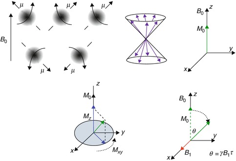
Fig. 4.2
The nuclear magnetic resonance phenomenon (clockwise) – protons abstracted as spinning spheres align themselves along or against a main magnetic field B 0 (polarization). They also process about the B 0 field and the vectors line up along the surface of a cone. The net effect is a resultant z magnetization M aligned along with B 0. When an external orthogonal radiofrequency field B 1 is applied along x, it causes M to tip away from the z-axis by a flip angle θ. The transverse component of M (M xy ) produces an induced voltage in a coil placed in the x–y plane and is the NMR signal
Any perturbed system tries to recover its equilibrium state – in this case, the equilibrium state is M being aligned with B 0. While precessing about B 0, the magnetization vector M exhibits two important properties that are the basis of image contrast in MRI – (1) the longitudinal component of M (M z ) grows exponentially with a time constant of T 1, referred to as spin–lattice relaxation time, and (2) the transverse component of M (M xy ) which is producing the MR signal decays exponentially with a time constant of T 2, referred to as spin-spin relaxation time. This is shown in Fig. 4.3. The equations governing the exponential behavior of these two components over time are called Bloch equations. Physically, T 1 refers to the transfer of energy from the excited spins to the lattice atoms, and T 2 refers to the loss of energy due to mutual interaction between the spins resulting in loss of phase coherence. The values of T 1 and T 2 differ for protons in different local magnetic environments and molecules giving rise to image contrast. For example, protons in lipid molecules exhibit a much shorter T 1 than free water protons in a cyst. The exponentially decaying signal induced by the coil is referred to as free induction decay (FID). T 1 also determines how often the experiment can be repeated, i.e., how often the B 1 RF pulse is applied and the time interval between applications of successive B 1 pulses is called repetition time (TR).
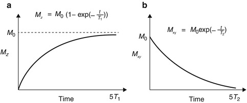
Fig. 4.3
Spin–lattice relaxation (T 1) and spin-spin relaxation (T 2) times – the parameter T 1 describes the recovery of the longitudinal magnetization M z to its equilibrium value M 0, while T 2 describes the decay of the transverse magnetization M xy . These parameters are different for different types of protons (e.g., protons in free water, bound water, and lipid) resulting in soft tissue contrast. The equations describing these relaxation times are also shown
Image Formation
The application of an external RF field B 1 to tip the magnetic moment M to the transverse plane produces only a “one-dimensional” signal that contains no spatial information about the object being imaged. In order to achieve spatial discrimination, magnetic field gradients are used. The application of a magnetic field gradient G x along the x-direction, for example, causes the main magnetic field B 0 to vary along x as B 0 + xG x, where x refers to the spatial coordinate. This causes spins along x to resonate in a range of frequencies centered around the Larmor frequency and linearly proportional to the distance of the spin from the isocenter of the bore (where the gradient strength is zero by design). By applying gradients along two directions x and y, a unique signal characterized by its unique frequency can be elicited as a function of x and y, which in essence is a two-dimensional image. In practice, a gradient is applied along the z direction to select a “slice.” In order to separate signals with different frequency components, a Fourier transform is applied in the x–y dimension. Magnetic field gradients can be applied along any direction, permitting image acquisition in arbitrary planes, a significant departure from the axial plane restriction of CT imaging.
Image Contrast
The time between the application of a B 1 RF pulse and center of data acquisition is called echo time (TE). This parameter along with the sequence repetition time (TR) is a strong determinant of MRI image contrast. The spin–lattice and spin-spin relaxation times T 1 and T 2 along with the spin (or proton) density are different for protons in different molecules (e.g., fat, gray matter, white matter) and environments, generating soft tissue contrast. In the human body, typical values of T 2 are 10–50 ms and T 1 100–1,500 ms. By changing the TE and TR, differences in T 1, T 2, or proton density (PD) can be highlighted, giving rise to T 1 -weighted, T 2 -weighted, or PD-weighted images, the three most common types of images acquired in MRI. T 2-weighted sequences are characterized by long TR and long TEs, while T1-weighted sequences usually employ short TRs and short TEs. Proton-density weighting can be elicited using long TRs and short TEs, minimizing both T 1 and T 2 effects.
MRI Hardware
The main components of an MRI system are shown in Fig. 4.4. The main magnetic field B 0 is created by winding a superconducting material around a cylindrical bore, which also houses the patient table. The superconducting material enables the sustenance of high currents, which are needed for producing strong magnetic fields (1–3 T), typically used in modern whole-body MRI systems. The RF coil that produces the excitation RF B 1 field is also integrated into the bore. The MRI signal is typically sensed using RF coils with differing geometries, tailored to the body part being imaged. A torso phased-array receive coil for abdominal imaging is shown here. The spatially varying magnetic field gradients are also integrated into the bore and produced by winding wires around a core. These gradients are situated in a different layer in the bore than the superconducting windings, which produce B 0. The signal detected by the RF coils are filtered, amplified, digitized, and then processed to generate the final MRI image.
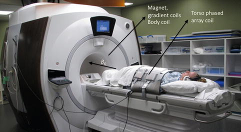
Fig. 4.4
A modern whole-body 3T MRI clinical scanner – the cylindrical bore houses the superconducting coil, which produces the main magnetic field (B 0), the gradient coils, as well as the body RF coil which excites the spins. MRI signal reception is performed using a torso phased-array coil designed for abdominal imaging and wrapped around the patient as shown (Image courtesy: Ann Sawyer, Stanford University)
Magnetic Resonance Urography (MRU)
MRU refers to the class of MRI techniques that are used for noninvasive anatomical and functional imaging of the kidneys and the urinary tract. MRU is often classified as static (fluid) and dynamic (excretory) urography. Static fluid MRU is T 2-weighted and performed without any contrast injection, while dynamic or excretory MRU is performed after injection of a gadolinium-based pharmacological contrast agent using a T1-weighted MR imaging sequence. Friedburg and associates first applied MRI to urography using a strongly T 2-weighted sequence to delineate the efferent urinary pathways in 1987 [6]. In most situations, static and dynamic MRU provide complementary information, leading to a more accurate diagnosis.
Static MR Urography
Static MRU is very useful for characterization of fluid-filled and dilated structures such as hydronephrosis, megaureters, cysts, ureteroceles, and similar pathologies. While it is very useful for obtaining anatomic information in patients with dilated or obstructed collecting systems, it is not very useful for eliciting functional information, especially in non-dilated systems. Because gadolinium contrast agents cause concomitant reduction of T 2 relaxation times in addition to T 1, static MRU is performed prior to injection of gadolinium-based contrast agents. In static MRU, the long T 2 relaxation time of urine is exploited for achieving T 2-weighting [7, 8]. A pulse sequence with a long echo time (TE) is used to suppress signal from background tissue, which have shorter T2 relaxation times. Fat suppression can also be used to further reduce background signal and improve conspicuity of structures of interest such as the ureters. In addition to thin section multi-slice 2D imaging, thick slab 2D imaging or even 3D T 2-weighted imaging sequences have been reported for use in static fluid MRU.
In order to minimize scan times and reduce motion artifacts from breathing and peristalsis, a half-Fourier single-shot imaging technique (called single-shot fast spin echo (SSFSE), rapid acquisition with relaxation enhancement (RARE), or single-shot turbo spin echo (TSE) by the main MRI vendors) is most commonly used in conjunction with breath-holding [8, 9]. Sometimes, respiratory gating is used to gate the acquisition to the quiescent period of the respiratory cycle and obviate the need for breath-holding. The use of respiratory-gated 3D spin echo sequences has also been reported but at the cost of increased scan times [10]. The use of variable refocusing flip angle 3D fast spin echo sequences (called Cube, SPACE, or VISTA by three of the main MRI vendors) can enable the use of long echo trains, which significantly reduces scan times. Three-dimensional imaging sequences enable the acquisition of volumes with thin section thicknesses, which can then be post-processed to yield maximum intensity projection (MIP) or volume rendered images for depiction of the entire urinary tract.
Dynamic MR Urography
Dynamic or excretory MRU is T 1 -weighted and performed after administration of a gadolinium-based contrast agent to follow its time course of uptake and excretion. This information can then be used to generate quantitative metrics of renal function such as renal and calyceal transit times, differential renal function, single-kidney GFRs, and even GFR maps. Due to the high vascularity of tumors, T 1-weighted MRI is also used in the detection and characterization of malignancies. Dynamic MRU is more useful in non-dilated systems but requires minimal renal function for excretion and redistribution of the contrast material, often enhanced by using a diuretic such as furosemide. This also causes dilution and redistribution of the contrast agent for optimal image quality and minimizes any signal loss from contrast agent pooling [11, 12].
A 3D spoiled gradient-echo sequence with fat suppression is used repeatedly to capture the signal time course to filling and excretion of urine [11, 13, 14]. This sequence is referred to as VIBE, THRIVE, or LAVA by the main MRI vendors. Fat suppression improves ureter conspicuity as in static MRU. The urine signal is bright due to the T 1 shortening produced by the contrast agent in conjunction with the T 1-weighted pulse sequence, which renders background dark due its longer T 1. A coronal 3D acquisition can be used to image the kidneys, ureters, and the bladder in a single plane. This sequence is typically acquired in a breath-hold if possible or using respiratory gating. Figure 4.5 shows an example of static MR urography (left) and dynamic MR urography (right) on a patient with a smaller left kidney and multiple cysts. The fluid-filled cysts are clearly visualized on the static T 2-weighted image, whereas the dynamic T 1-weighted image shows the cortical enhancement and the lack of enhancement of the cysts. The dynamic 3D T 1-weighted sequence used respiratory triggering to acquire each 3D volume in about 12 s.
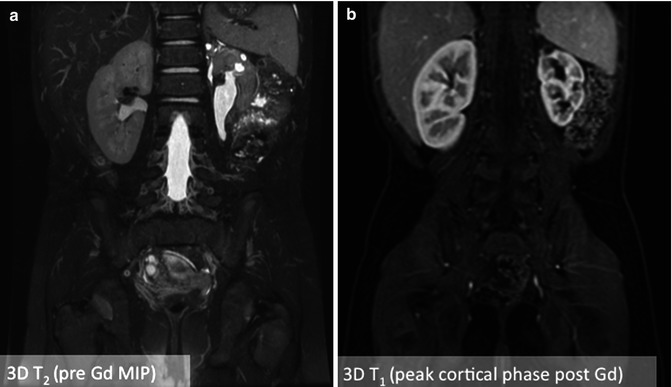
Fig. 4.5
An example of static MR urography (left) versus dynamic MR urography (right) images from a patient with a slightly atrophied left kidney and multiple cysts. The fluid-filled cysts are clearly visualized on the static 3D T2-weighted image, whereas the dynamic 3D T 1-weighted image acquired 30 s after injection of gadolinium contrast shows peak cortical enhancement and lack of cystic enhancement
Contrast Agents
Gadolinium is a heavy metal in the lanthanide series and is widely used in MRI as an intravenous contrast agent after chelating it with various ligands, most commonly DTPA (Gd-DTPA), to render it safe. A paramagnetic ion with a large magnetic moment due to its seven unpaired electrons, even in very small amounts, gadolinium reduces the T 1 and T 2 of the water protons it comes in close proximity to. The amount of T 1 shortening is linearly proportional to the concentration of contrast agent present for the range of typical in vivo concentrations. Gadolinium chelates exhibit pharmacokinetic properties very similar to that of iodinated contrast agents – they disperse readily into intravascular and extracellular compartments and are excreted by glomerular filtration. The T 1-shortening property of Gd-DTPA and similar contrast agents make it attractive for T 1-weighted imaging. In dynamic MRU, imaging is performed repeatedly following administration of the contrast agent.
In order to extract quantifiable measures of renal function, the MRI signal intensity is used as a surrogate for contrast agent concentration. This approximation is valid only at low concentrations of gadolinium contrast typically 0.1 mmol/kg. In MRU, since urine can concentrate in structures especially when there is an obstruction, the gadolinium concentration can also become very high resulting in signal loss due to T 2* effects. As a result, concentrations as low as 0.025 mmol/kg are used. An accurate way of estimating the contrast agent concentration from MRI signal intensity is using the knowledge of T 1 prior to injection acquired using a T 1-mapping technique. The most commonly used T 1-mapping technique is to image using a pure T 1-weighted imaging sequence such as 3D spoiled gradient echo with multiple flip angles. The T 1 values can then be estimated using a parametric fitting. The change in T 1 can then be used to calibrate the contrast agent concentration, as the signal dependency on T 1 is known a priori [15].
Elements of a Typical MRU Examination
A typical MRU exam comprises of four main steps: (a) patient preparation, (b) data acquisition, (c) image processing, and (d) modeling. While the first two steps are absolutely essential to extract any functional information from the dynamic MRU examination, the last step of modeling is usually performed only if a fully quantitative parametric modeling is desired. The image-processing step is used to segment out the aorta, collecting systems, medulla, and cortex for the individual kidneys. These steps are summarized in Fig. 4.6. The segmented cortex and medulla for each kidney are depicted in different colors. After this segmentation step performed for the images at each time point, semiquantitative measures such as renal and calyceal transit times, volumes of the segmented compartments, relative signal enhancement curves, and differential renal function can be computed. The images can be processed further to extract single-kidney GFRs, medullary and cortical GFRs, or pixel-wise GFR maps using modeling techniques. Many groups use basic image processing to segment and extract semiquantitative parameters instead of modeling the contrast uptake using complex parametric models.
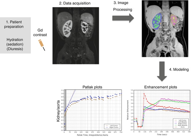
Fig. 4.6
Elements of a typical MRU exam illustrating the key steps of patient preparation, data acquisition (imaging), image processing, and modeling. The image-processing step is used to segment the kidney into medulla, cortex, and collecting system (color coded here) to generate separate cortical and medullary GFR measurements
Patient Preparation
Patient preparation is a critical aspect to obtaining reliable MRU quality. Most subjects under 6 years of age require sedation or anesthesia. A recent serum creatinine should be sought to estimate GFR. At our institution, a GFR less than 30 mL/min/m 2 precludes administration of gadolinium. Intravenous access with at least a 22 gauge peripheral IV is required; with 20 gauge preferred in older children. Thirty minutes prior to the start of image acquisition, a 20 mL/kg intravenous bolus of saline or lactated Ringers is administered, though this may be decreased on a case-by-case basis in patients’ cardiac or respiratory conditions that require restricted fluid intake. Once the bolus is complete, maintenance fluids of 10 mL/kg/h are continued until the completion of image acquisition. Additionally, a urinary bladder catheter is placed to ensure an empty bladder for physiologic reasons as well as to ensure the patient does not have to prematurely terminate the exam to void.
It is important that gadolinium contrast be diluted and dispersed in the collecting systems for optimal visualization as well as to minimize signal loss due to T 2* effects that can result from the pooling of gadolinium. As a result, dynamic MRU is almost always preceded by administration of a diuretic agent such as furosemide. This enhances the urinary flow and distribution of gadolinium within the collecting systems for optimal visualization.
Image Acquisition
Figure 4.7 summarizes a typical MRU protocol performed at our institution on a child with crossed fused renal ectopia. The top panel shows a 3D T 2-weighted image (a), a non-contrast angiography MIP image obtained using a 3D balanced SSFP sequence with an inversion recovery prep to suppress the background and venous signal (b) and a single frame from a multiphasic 2D balanced SSFP sequence (c). The remaining images (d–h) are from a respiratory-gated 3D T1-weighted sequence with Dixon fat-water separation obtained before injection of gadolinium contrast (d) and post-contrast (e–h) depicting peak cortical enhancement (e), peak medullary enhancement (f), late enhancement (g), and excretory phase with enhanced collecting system (h).
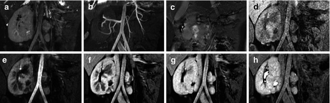
Fig. 4.7
Representative images from a typical MRU protocol performed at our institution on a child with crossed fused renal ectopia. Panels a–c show a 3D T 2-weighted image (a), a non-contrast angiography MIP image obtained using a 3D balanced SSFP sequence with an inversion recovery prep (b), a single frame from a multiphasic 2D balanced SSFP sequence (c). Pre-contrast (d) and post-contrast (e–h) phases from a respiratory-gated 3D T 1-weighted sequence with Dixon fat-water separation depict peak cortical enhancement (e), peak medullary enhancement (f), late enhancement, (g) and excretory phase with enhanced collecting system (h)
Image Processing
The data acquired in dynamic MRU is essentially a four-dimensional data set (i.e., a 3D volume as function of time). A number of quantitative metrics are extracted from these dynamic MRU images, which provide information about renal function. These metrics are computed pixel by pixel over the entire imaging volume or on the signal integrated over a user-specified region of interest (ROI). Commonly used metrics include calyceal transit time (CTT, the time taken for the contrast agent to reach the renal pelvis), renal transit time (RTT, the time between arrival of the contrast agent in the cortex and in the ureters), degree of enhancement (the maximum signal enhancement after injection of gadolinium contrast relative to the unenhanced signal expressed as a % and sometimes also calculated as a ratio to remove effects such as coil shading), time to peak (time taken to reach maximum degree of enhancement), maximal slope of enhancement, and differential renal function (maximum slope or area under the signal enhancement curve normalized by renal volume).
The features of interest in the 3D images are segmented first prior to extraction of parameters [16]. Simple image-processing techniques like image thresholding and more complex morphological operations like erosion and dilation are used to extract and label the aorta, left and right medullae, cortices, and the left and right collecting systems. These steps may be time-consuming requiring manual input for identification of the regions as well as readjustment if the image contrast is poor. Time-to-peak maps can assist in segmentation by identifying the image phase with the brightest signal in the region of interest and speed up the segmentation process. Signal from the aorta is used by most modeling-based approaches to compute the arterial input function. Medullary and cortical volumes can be computed for each kidney and used for normalization of split or differential renal function measures. In highly dilated or atrophied kidneys, it may not be possible to achieve this medullary-cortical segmentation, and it is customary to lump them together. Figure 4.8 shows two examples where the image segmentation was complicated by an atrophic kidney or a hydronephrotic kidney. Phased-array coils often produce nonuniform intensity variations across the image and can be corrected using vendor-supplied software, which removes any coil-induced variations in image intensity across the image.
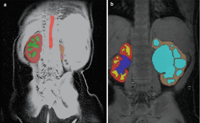
Fig. 4.8


Image segmentation results from a patient with an atrophic left kidney (left) and hydronephrosis (right), which make segmentation of the kidney into distinct cortical and medullary compartments difficult
Related posts:
Stay updated, free articles. Join our Telegram channel
Full access? Get Clinical Tree
