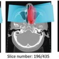
Robust Segmentation of Challenging Lungs in CT Using Multi-stage Learning and Level Set Optimization

Fig. 8.1

Examples of how diseases, such as tumors or interstitial lung disease, affect the appearance of lung in CT

In this article, we address the automatic segmentation of challenging cases described above and illustrated in Fig. 8.1. We first review the basic algorithms for segmenting healthy lung parenchyma and demonstrate the limitations of these algorithms in the presence of pathologies (Section “Segmenting Healthy Lungs”). We then discuss how texture cues, anatomical information, and statistical shape models, have been leveraged to improve robustness in the presence of disease. This is followed by the presentation of a method that utilizes machine learning with both texture cues and anatomical information from outside the lung to obtain a robust lung segmentation that is further improved with level set refinement (Section “Multi-Stage Learning for Lung Segmentation”). These algorithms are implemented in a modular software framework that promotes reuse and experimentation (Section “A Software Architecture for Detection and Segmentation”).

Segmenting Healthy Lungs

As healthy lung parenchyma has lower attenuation than the surrounding tissue, simple image processing techniques often achieve good results. The attenuation of healthy lung tissue in CT varies across the lung, depends on the phase of respiratory cycle [25] and image acquisition settings [2], with mean values being around − 860 to − 700 HU [25]. However, as illustrated in Fig. 8.2, the intensity distribution within the lung region is often completely disjoint from that of the higher density body tissue. Thus simple image processing operations, such as region growing, edge tracking [10], or simple thresholding [4, 11, 23], can be used to separate lung from body tissue.

Fig. 8.2

Healthy lung tissue is easily separable from body tissue with a single threshold

For example, thresholding methods first separate body tissue from surrounding background tissue by removing large connected components touching the edges of the images. Lung tissue can then be separated from the body tissue with a threshold. Hu et al. propose to use a dynamic threshold, τ, that is iteratively updated to be the mean of the average intensities between the lung and body, $\tau _{t} = (\mu _{\mathrm{ lung}}^{t-1} +\mu _{ \mathrm{ body}}^{t-1})/2$ , where μ _lung ^tand μ _body ^tare the mean HU values of the lying below and above τ _t, respectively [11]. The initial threshold, τ ₀, is estimated with $\mu _{\mathrm{ lung}}^{0} = -1,000$ and μ _body ⁰ is the average intensity of all HU values greater than 0.

Depending on the application, the final step is to separate the segmented lung tissue into left and right lungs. The thresholded lung regions are connected by the trachea and large airways and can be separated by region growing a trachea segmentation from the top of the segment [11, 39]. Further, the lungs often touch at the anterior and posterior junctions and need to be separated using another post-process that uses a maximum cut path to split the single lung component into the individual lungs [4, 11, 26].

The simple thresholding scheme gives a good gross estimate to the lung volume but often excludes small airways and vessels that a clinician would include with the lung annotation. These small regions can be filled through the use of morphological operations [11, 36], or by performing connected component analysis on the image slices [39] (see Fig. 8.3).

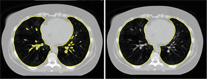
Fig. 8.3

Segmentation by simple thresholding often excludes airways and vessels (left). These vessels are easily removed by morphological operations or by removing small connected components on 2D slices (right)

Another subtle problem comes with nodules that lie on the boundary of the lung [27]. A complete segmentation of the lung is essential for cancer screening applications [3], and studies on computer aided diagnosis have found the exclusion of such nodules to be a limitation of automated segmentation and nodule detection methods [1]. These nodules can be included in the segmentation through the use of special post-processing steps, such as the adaptive border marching algorithm [23], which tries to include small concave regions on the lung slices. However, such algorithmic approaches are bound to fail for larger tumors whose size and shape are unconstrained (Fig. 8.4).

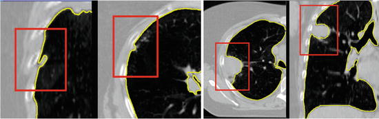
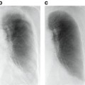
Fig. 8.4

Small juxtapleural nodules like those in the left figure can be included in the final segmentation through the use of morphological operations, but finding a set of parameters to include all possible tumors, such as those in the cases on the right, is challenging

Even more problematic is interstitial lung disease, which causes a dramatic change in the attenuation and local texture pattern of lung parenchyma. Unlike the clearly separated histograms of healthy lung (Fig. 8.3), such diseased tissue will often have attenuation values that overlap with the surrounding body tissue (Fig. 8.5). Although higher thresholds, such as − 300 HU [39], can be used to include more lung tissue, simple thresholding methods are incapable of robustly segmenting these challenging pathologies.

Fig. 8.5

Lungs with diffuse pulmonary disease has higher density tissue and is difficult to separate with a simple thresholding

Cues for Segmenting Pathological Lung

Intensity alone is the single strongest cue for segmenting healthy lung tissue, but in order to address the high density lung tissue associated with interstitial lung disease, and the different shapes associated with varying tumors, cues based on texture, anatomy, or shape priors must be exploited.

Texture Cues

Diseased parenchyma has a different texture pattern which can often be extracted through the use of texture features [20, 37, 39]. Texture, the local structural pattern of intensities, is commonly characterized by measurements obtained from a co-occurrence matrix [9], which records the joint frequency of intensity values between two pixels separated by a fixed offset computed over small volumes of interest around each image voxel. Quantities derived from this co-occurrence matrix, such as entropy, can be used to directly identify diseased tissue [39], or statistical classifiers can be trained to distinguish healthy from pathological tissue using features derived from this matrix [37].

Anatomical Cues

As the appearance of the pathological lung parenchyma can vary dramatically, texture and intensity cues are incapable of capturing all pathologies. These quantities, which are internal to the lung, can be combined with neighboring anatomical context, such as distance and curvature of the ribs. For example, Prasad et al. use the curvature of the ribs in order to adaptively choose a threshold for the lung segmentation [22]. As the lung border should also lie close to the ribcage and spine, distance to these anatomical structures can be combined with intensity features in classification of the lung border [12].

Shape Modeling

In order to avoid segmentations with unlikely shapes, such as the one in Fig. 8.5, a shape prior can be used as an additional cue for segmenting challenging cases. Although some inconsistencies in the shape can be removed, for example, by post-processing operations [11] or through ensuring smoothness in the resulting segmentations [12], the result should be constrained to be lung-like. Explicit statistical models of shape variability, such as a point distribution model that models the shape variability with a low-dimensional linear subspace can be used to constrain the resulting segmentation [6]. These models have been effectively used to overcome pathologies [30, 32].

Segmentation-by-registration are another class of methods that enforce a prior constraint on the resulting segmentations. In such approaches, a reference image complete with annotations is aligned to the target image through the process of image alignment. The target segmentation is then derived from the aligned reference image. To increase generality, multiple reference images can be aligned to the target image and the final segmentation can be taken as the fused result. Depending on the matching score used in the registration, such methods have shown to be effective for pathological lungs [28].

Multi-stage Learning for Lung Segmentation

To ensure robustness, a complete solution to the segmentation of pathological lung in CT has to include components that address shape and appearance variability caused by both tumors and diffuse lung disease. In this section we introduce a robust machine learning method for segmenting challenging lung cases that uses external anatomical information to position a statistical mesh model on the image. A large database of annotated images is used to train discriminative classifiers to detect initial poses of the mesh models and to identify stable boundary landmarks [30]. The boundary of this initialization is then guided by texture and appearance patterns to identify the boundary of the lung. Finally, as pathologies often only occupy a small portion of the lung, a fine-scale level set surface refinement is used to ensure the final segmentation includes all healthy regions as well as preserving the segmentation in the pathological regions [18]. The elements of the system are illustrated in Fig. 8.6.

Fig. 8.6

A hierarchical detection network is used to initialize the lung segmentations from a set of stable landmarks. These segmentations are further refined by trained boundary detectors and finally by a fine-scale level set refinement

Learning-Based Robust Initialization

For the initialization phase, the carina of the trachea is detected in the input volume. Given the carina location, a Hierachical Detection Network (HDN) [31] is used to detect an initial set of pose parameters of statistical shape models of each lung (Sections “Hierarchical Detection Network” and “Pose Detection”). In the next level of the hierarchy, stable landmark points on the mesh surface are refined to get an improved lung segmentation that is less sensitive to appearance changes within pathologies (Section “Refinement Using Stable Landmarks”). As we will see, these landmark points tend to use nearby anatomical context, e.g., ribs, to improve the segmentation. A further refinement comes by displacing the mesh surface so as to maximize the score of an appearance-based classifier (Section “Freeform Refinement”).

Input Annotation Database

A set of CT images complete with manual annotation of the lungs is used as input to the algorithm. In an offline training step, statistical shape models of the shape variation within the database annotations are learned.

The input annotation meshes are first brought into correspondence and remeshed so that each annotation mesh has the same number of points and a consistent triangulation. Each annotation mesh, $\mathcal{M}_{k} = (\mathcal{P}_{k},\mathcal{T} )$ , then consists of a set of points, $\mathcal{P}_{k} =\{ \mathbf{v}_{ki} \in {\mathbb{R}}^{3}\}_{i=1}^{N}$ , and a single set of triangle indices, $\mathcal{T} =\{ \bigtriangleup _{j} \in {\mathbb{Z}}^{3}\}_{j=1}^{N_{tri}}$ .

The variability in the point coordinates is modeled through a low-dimensional linear basis giving a statistical shape model,

$\displaystyle{ {\mathcal{C}} = (\{{\bf \hat{ v}}\}_{i=1}^{N},\{U_{ j}\}_{j=1}^{M}), }$

(8.1)

that consists of a mean shape, $\{{\bf \hat{ v}}\}_{i=1}^{N}$ , and the linear basis shapes, $U_{j} =\{ u_{ij}\}_{i=1}^{N}$ . The linear basis is empirically estimated by performing PCA on the aligned input annotation meshes. The alignment uses procrustes analysis to remove translation, orientation, and scale variation of the corresponding meshes.

A mesh in the span of the basis can be approximated by modulating the basis shape vectors and applying a similarity transform

$\displaystyle{ g({\bf v}_{i};\{\lambda _{j}\},{\bf p},{\bf r},{\bf s}) = {\bf p} + {\bf M}({\bf s},{\bf r})\sum _{j}\left ({\bf \hat{ v}}_{i} + {\bf u}_{ij}\lambda _{j}\right ), }$

(8.2)

where M(s, r) is the rotation and scale matrix parameterized by rotation angles, r, and anisotropic scale, s. p is a translation vector, and {λ _j} are the shape coefficients. Figure 8.7 illustrates the variability encoded by the first three basis vectors for a model of the right lung.

Fig. 8.7

The variability of right lung shape model by using one of the first three basis vectors to represent the shape

Each training shape can be approximated in the same manner, meaning each training shape has an associated pose and shape coefficient vector. In the following description of the image-based detection procedure, the relationship between these pose and shape coefficients and the image features is modeled with machine learning so that the parameters of the shape model can be inferred on unseen data.

Hierarchical Detection Network

The Hierarchical Detection Network (HDN) uses an efficient sequential decision process to estimate the unknown states (e.g., object poses or landmark positions) of a sequence of objects that depend on each other [31]. In the case of lung segmentation, the unknown states are the poses and shape coefficients that align a statistical model of the lung to the image, which depend on the detected trachea landmark point. The location of stable lung boundary points are dependent on the pose parameters of the lungs.

The HDN infers multiple dependent object states sequentially using a model of the prior relationship between these objects. Let θ _tdenote the unknown state of an object (e.g., the 9 parameters of a similarity transform or the 3D coordinates of a landmark), and let the complete state for t + 1 objects, θ ₀, θ ₁, …, θ _t, be denoted as θ _0:t. Given a d-dimensional input volume, V : ℝ ^d↦ ℝ, the estimation for each object, t, uses an observation region V _t ⊆ V. The complete state is inferred from the input volume by maximizing the posterior density, f(θ _0:t|V _0:t), which is recursively decomposed into a product of individual likelihoods, f(V _t|θ _t), and the transition probability between the objects, f(θ _t|θ _0:t−1).

The recursive decomposition of the posterior is derived by applying a sequence of prediction and update steps. For object t, the prediction step ignores the observation region, V _t, and approximates the posterior, f(θ _0:t|V _0:t−1), using a product of the transition probability, f(θ _t|θ _0:t−1), and the posterior of the preceding objects:

$\displaystyle\begin{array}{lll} f({\boldsymbol{\theta} }_{0:t}\vert V _{0:t-1})& = f({\boldsymbol{\theta} }_{t}\vert {\boldsymbol{\theta} }_{0:t-1},V _{0:t-1})f({\boldsymbol{\theta} }_{0:t-1}\vert V _{0:t-1}),&{}\end{array}$

(8.3)

$\displaystyle\begin{array}{lll} &\quad\quad = f({\boldsymbol{\theta}}_{t}\vert {\boldsymbol{\theta} }_{0:t-1})f({\boldsymbol{\theta} }_{0:t-1}\vert V _{0:t-1}),&{}\end{array}$

(8.4)

as θ _tand V _{0: t − 1} are assumed to be conditionally independent given θ _{0:t − 1}.

The observation region, V _t, is then combined with the prediction in the update step,

$\displaystyle\begin{array}{lll} f({\boldsymbol{\theta} }_{0:t}\vert V _{0:t})& = \frac{f(V _{0:t}\vert {\boldsymbol{\theta} }_{0:t})f({\boldsymbol{\theta} }_{0:t})} {f(V _{0:t})} = \frac{f(V _{t}\vert V _{0:t-1},{\boldsymbol{\theta} }_{0:t})f(V _{0:t-1}\vert {\boldsymbol{\theta} }_{0:t})f({\boldsymbol{\theta} }_{0:t})} {f(V _{t}\vert V _{0:t-1})f(V _{0:t-1})} &{}\end{array}$

(8.5)

$\begin{array}{lll} & = \frac{f(V _{t}\vert {\boldsymbol{\theta} }_{t})f({\boldsymbol{\theta} }_{0:t}\vert V _{0:t-1})} {f(V _{t}\vert V _{0:t-1})} ,&{}\end{array}$

(8.6)

where the denominator is a normalizing term, and the derivation assumes V _tand $(V _{0:t-1},{\boldsymbol{\theta} }_{0:t-1})$ are conditionally independent given θ _t. The likelihood term, f(V _t|θ _t), is modeled with a discriminative classifier,

$\displaystyle{ f(V _{t}\vert {\boldsymbol{\theta} }_{t}) = f(y = +1\vert V _{t},{\boldsymbol{\theta} }_{t}), }$

(8.7)

where the random variable y∈{ − 1, 1} denotes the occurrence of the t ^th object at pose θ _t. The posterior, $f(y = +1\vert V _{t},{\boldsymbol{\theta} }_{t})$ , is modeled with a powerful tree-based classifier, the Probabilistic Boosting Tree (PBT) [33], which is trained to predict the label, y, given the observation region, V _tand a state, θ _t.

The prediction step models the dependence between the objects with the transition prior. In the case of lung segmentation, each object is dependent on one of the previous objects, meaning

$\displaystyle{ f({\boldsymbol{\theta} }_{t}\vert {\boldsymbol{\theta} }_{0:t-1}) = f({\boldsymbol{\theta} }_{t}\vert {\boldsymbol{\theta} }_{j}),\ \ \exists j \in \{ 0,1,2, \ldots ,t - 1\}. }$

(8.8)

The relation between the objects, f(θ _t | θ _j), is modeled using a Gaussian distribution whose parameters are learned from training data. In our application, the poses of each lung are dependent on the initial carina landmark point (Fig. 8.6). The stable landmarks, which are distributed on the boundary of the lungs, are then dependent on the pose of the lung.

The full posterior, f(θ _0:t | V _0:t), is approximated through sequential importance sampling, where a set of weighted particles (or samples), {θ _t^j, w _t^j}P _j=1, is used to approximate the posterior at state t, and these particles are propagated, in sequence, to the next object (see [31] for more details).

Pose Detection

The pose of each lung is represented with a 9-dimensional state vector, θ _t = {p _t, r _t, s _t}, containing a translation vector p ∈ ℝ ³, Euler angles for orientation r, and an anisotropic scale, s. The 9 pose parameters are decomposed into three sequential estimates of the respective 3-dimensional quantities [21, 42

Only gold members can continue reading. Log In or Register to continue