from only 30 samples (indicated by the red dots in Fig. 1b). From a first look at the time-domain signal, one would rather believe that reconstruction should be impossible from only 30 samples. Indeed, the spectrum reconstructed by traditional ℓ 2-minimization is very different from the true spectrum. Quite surprisingly, ℓ 1-minimization performs nevertheless an exact reconstruction, that is, with no recovery error at all!
Fig. 1
(a) 10-sparse Fourier spectrum, (b) time-domain signal of length 300 with 30 samples, (c) reconstruction via ℓ 2-minimization, (d) exact reconstruction via ℓ 1-minimization
An example from nuclear magnetic resonance imaging serves as a second illustration. Here, the device scans a patient by taking 2D or 3D frequency measurements within a radial geometry. Figure 2a describes such a sampling set of a 2D Fourier transform. Since a lengthy scanning procedure is very uncomfortable for the patient, it is desired to take only a minimal amount of measurements. Total variation minimization, which is closely related to ℓ 1-minimization, is then considered as recovery method. For comparison, Fig. 2b shows the recovery by a traditional back-projection algorithm. Figure 2c, d displays iterations of an algorithm, which was proposed and analyzed in [72] to perform efficient large-scale total variation minimization. The reconstruction in Fig. 2d is again exact!
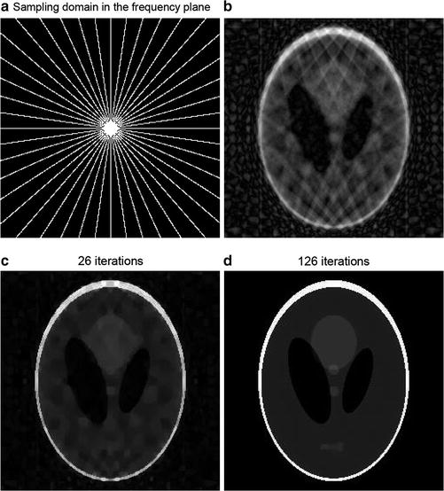
Fig. 2
(a) Sampling data of the NMR image in the Fourier domain which corresponds to only 0. 11 % of all samples. (b) Reconstruction by back projection. (c) Intermediate iteration of an efficient algorithm for large-scale total variation minimization. (d) The final reconstruction is exact
2 Background
Although the term compressed sensing (compressive sensing) was coined only recently with the paper by Donoho [47], followed by a huge research activity, such a development did not start out of thin air. There were certain roots and predecessors in application areas such as image processing, geophysics, medical imaging, computer science, as well as in pure mathematics. An attempt is made to put such roots and current developments into context below, although only a partial overview can be given due to the numerous and diverse connections and developments.
Early Developments in Applications
Presumably the first algorithm which can be connected to sparse recovery is due to the French mathematician de Prony [127]. The so-called Prony method, which has found numerous applications [109], estimates nonzero amplitudes and corresponding frequencies of a sparse trigonometric polynomial from a small number of equispaced samples by solving an eigenvalue problem. The use of ℓ 1-minimization appears already in the Ph.D. thesis of B. Logan [106] in connection with sparse frequency estimation, where he observed that L 1-minimization may recover exactly a frequency-sparse signal from undersampled data provided the sparsity is small enough. The paper by Donoho and Logan [52] is perhaps the earliest theoretical work on sparse recovery using L 1-minimization. Nevertheless, geophysicists observed in the late 1970s and 1980s that ℓ 1-minimization can be successfully employed in reflection seismology where a sparse reflection function indicating changes between subsurface layers is sought [140, 148]. In NMR spectroscopy the idea to recover sparse Fourier spectra from undersampled non-equispaced samples was first introduced in the 1990s [158] and has seen a significant development since then.
In image processing the use of total variation minimization, which is closely connected to ℓ 1-minimization and compressive sensing, first appears in the 1990s in the work of Rudin, Osher, and Fatemi [139] and was widely applied later on. In statistics where the corresponding area is usually called model selection, the use of ℓ 1-minimization and related methods was greatly popularized with the work of Tibshirani [149] on the so-called LASSO (Least Absolute Shrinkage and Selection Operator).
Sparse Approximation
Many lossy compression techniques such as JPEG, JPEG-2000, MPEG, or MP3 rely on the empirical observation that audio signals and digital images have a sparse representation in terms of a suitable basis. Roughly speaking one compresses the signal by simply keeping only the largest coefficients. In certain scenarios such as audio signal processing, one considers the generalized situation where sparsity appears in terms of a redundant system – a so-called dictionary or frame [36] – rather than a basis. The problem of finding the sparsest representation/approximation in terms of the given dictionary turns out to be significantly harder than in the case of sparsity with respect to a basis where the expansion coefficients are unique. Indeed, in [108, 114], it was shown that the general ℓ 0-problem of finding the sparsest solution of an underdetermined system is NP-hard. Greedy strategies such as matching pursuit algorithms [108], FOCUSS [86] and ℓ 1-minimization [35] were subsequently introduced as tractable alternatives. The theoretical understanding under which conditions greedy methods and ℓ 1-minimization recover the sparsest solutions began to develop with the work in [50, 51, 62, 78, 81, 87, 151, 152].
Information-Based Complexity and Gelfand Widths
Information-based complexity (IBC) considers the general question of how well a function f belonging to a certain class  can be recovered from n sample values or, more generally, the evaluation of n linear or nonlinear functionals applied to f [150]. The optimal recovery error which is defined as the maximal reconstruction error for the “best” sampling method and “best” recovery method (within a specified class of methods) over all functions in the class
  is closely related to the so-called Gelfand width of
  [38, 47, 117]. Of particular interest for compressive sensing is
  , the ℓ 1-ball in
  since its elements can be well approximated by sparse ones. A famous result due to Kashin [96] and Gluskin and Garnaev [79, 84] sharply bounds the Gelfand widths of B 1 N (as well as their duals, the Kolmogorov widths) from above and below; see also [77]. While the original interest of Kashin was in the estimate of n-widths of Sobolev classes, these results give precise performance bounds in compressive sensing on how well any method may recover (approximately) sparse vectors from linear measurements [38, 47]. The upper bounds on Gelfand widths were derived in [96] and [79] using (Bernoulli and Gaussian) random matrices (see also [107]), and in fact such type of matrices have become very useful also in compressive sensing [26, 47].
can be recovered from n sample values or, more generally, the evaluation of n linear or nonlinear functionals applied to f [150]. The optimal recovery error which is defined as the maximal reconstruction error for the “best” sampling method and “best” recovery method (within a specified class of methods) over all functions in the class is closely related to the so-called Gelfand width of [38, 47, 117]. Of particular interest for compressive sensing is , the ℓ 1-ball in since its elements can be well approximated by sparse ones. A famous result due to Kashin [96] and Gluskin and Garnaev [79, 84] sharply bounds the Gelfand widths of B 1 N (as well as their duals, the Kolmogorov widths) from above and below; see also [77]. While the original interest of Kashin was in the estimate of n-widths of Sobolev classes, these results give precise performance bounds in compressive sensing on how well any method may recover (approximately) sparse vectors from linear measurements [38, 47]. The upper bounds on Gelfand widths were derived in [96] and [79] using (Bernoulli and Gaussian) random matrices (see also [107]), and in fact such type of matrices have become very useful also in compressive sensing [26, 47]. Compressive Sensing
The numerous developments in compressive sensing began with the seminal work [30, 47]. Although key ingredients were already in the air at that time, as mentioned above, the major contribution of these papers was to realize that one can combine the power of ℓ 1-minimization and random matrices in order to show optimal results on the ability of ℓ 1-minimization of recovering (approximately) sparse vectors. Moreover, the authors made very clear that such ideas have strong potential for numerous application areas. In their work [26, 30] Candès, Romberg, and Tao introduced the restricted isometry property (which they initially called the uniform uncertainty principle) which is a key property of compressive sensing matrices. It was shown that Gaussian, Bernoulli, and partial random Fourier matrices [26, 129, 138] possess this important property. These results require many tools from probability theory and finite-dimensional Banach space geometry, which have been developed for a rather long time now; see, e.g., [95, 103].
Donoho [49] developed a different path and approached the problem of characterizing sparse recovery by ℓ 1-minimization via polytope geometry, more precisely, via the notion of k-neighborliness. In several papers sharp phase transition curves were shown for Gaussian random matrices separating regions where recovery fails or succeeds with high probability [49, 53, 54]. These results build on previous work in pure mathematics by Affentranger and Schneider [2] on randomly projected polytopes.
Developments in Computer Science
In computer science the related area is usually addressed as the heavy hitters detection or sketching. Here one is interested not only in recovering signals (such as huge data streams on the Internet) from vastly undersampled data, but one requires sublinear runtime in the signal length N of the recovery algorithm. This is no impossibility as one only has to report the locations and values of the nonzero (most significant) coefficients of the sparse vector. Quite remarkably sublinear algorithms are available for sparse Fourier recovery [80]. Such algorithms use ideas from group testing which date back to World War II, when Dorfman [56] invented an efficient method for detecting draftees with syphilis.
In sketching algorithms from computer science, one actually designs the matrix and the fast algorithm simultaneously [42, 82]. More recently, bipartite expander graphs have been successfully used in order to construct good compressed sensing matrices together with associated fast reconstruction algorithms [11].
3 Mathematical Modelling and Analysis
This section introduces the concept of sparsity and the recovery of sparse vectors from incomplete linear and nonadaptive measurements. In particular, an analysis of ℓ 1-minimization as a recovery method is provided. The null space property and the restricted isometry property are introduced, and it is shown that they ensure robust sparse recovery. It is actually difficult to show these properties for deterministic matrices and the optimal number m of measurements, and the major breakthrough in compressive sensing results is obtained for random matrices. Examples of several types of random matrices which ensure sparse recovery are given, such as Gaussian, Bernoulli, and partial random Fourier matrices.
Preliminaries and Notation
This exposition mostly treats complex vectors in  although sometimes the considerations will be restricted to the real case
  . The ℓ p -norm of a vector
  is defined as
For 1 ≤ p ≤ ∞, it is indeed a norm, while for 0 < p < 1, it is only a quasi-norm. When emphasizing the norm, the term ℓ p N is used instead of  or
or  . The unit ball in ℓ p N is
  . The operator norm of a matrix
  from ℓ p N to ℓ p m is denoted
In the important special case p = 2, the operator norm is the maximal singular value σ max(A) of A.
although sometimes the considerations will be restricted to the real case . The ℓ p -norm of a vector is defined as(1)
or . The unit ball in ℓ p N is . The operator norm of a matrix from ℓ p N to ℓ p m is denoted(2)
For a subset  , one denotes by
  the vector which coincides with
  on the entries in T and is zero outside T. Similarly, A T denotes the column submatrix of A corresponding to the columns indexed by T. Further,
  denotes the complement of T and # T or | T | indicates the cardinality of T. The kernel of a matrix A is denoted by
  .
.
, one denotes by the vector which coincides with on the entries in T and is zero outside T. Similarly, A T denotes the column submatrix of A corresponding to the columns indexed by T. Further, denotes the complement of T and # T or | T | indicates the cardinality of T. The kernel of a matrix A is denoted by .Sparsity and Compression
Compressive sensing is based on the empirical observation that many types of real-world signals and images have a sparse expansion in terms of a suitable basis or frame, for instance, a wavelet expansion. This means that the expansion has only a small number of significant terms, or, in other words, that the coefficient vector can be well approximated with one having only a small number of nonvanishing entries.
The support of a vector x is denoted  and
and
 It has become common to call
  the ℓ 0-norm, although it is not even a quasi-norm. A vector x is called k–sparse if
  . For
. For  ,
,
 denotes the set of k-sparse vectors. Furthermore, the best k -term approximation error of a vector
  in ℓ p is defined as
 If σ k (x) decays quickly in k, then x is called compressible. Indeed, in order to compress x, one may simply store only the k largest entries. When reconstructing x from its compressed version, the non-stored entries are simply set to zero, and the reconstruction error is σ k (x) p . It is emphasized at this point that the procedure of obtaining the compressed version of x is adaptive and nonlinear since it requires the search of the largest entries of x in absolute value. In particular, the location of the nonzeros is a nonlinear type of information.
and the ℓ 0-norm, although it is not even a quasi-norm. A vector x is called k–sparse if . For , in ℓ p is defined asThe best k -term approximation of x can be obtained using the nonincreasing rearrangement  , where i j denotes a permutation of the indexes such that
  for
for  . Then it is straightforward to check that
 And the vector x [k] derived from x by setting to zero all the N − k smallest entries in absolute value is the best k -term approximation,
![$$\displaystyle{x_{[k]} =\arg \min _{z\in \Sigma _{k}}\|x - z\|_{p},}$$](/wp-content/uploads/2016/04/A183156_2_En_6_Chapter_Eque.gif) for any 0 < p ≤ ∞.
for any 0 < p ≤ ∞.
, where i j denotes a permutation of the indexes such that for . Then it is straightforward to check thatThe next lemma states essentially that ℓ q -balls with small q (ideally q ≤ 1) are good models for compressible vectors.
Lemma 1.
Let 0 < q < p ≤∞ and set  . Then
. ThenProof.
Let T be the set of indexes of the k-largest entries of x in absolute value. The nonincreasing rearrangement satisfies | r k (x) | ≤ | x j | for all j ∈ T, and therefore
 Hence,
  . Therefore,
 which implies
  ■
■
. Therefore, ■Compressive Sensing
The above outlined adaptive strategy of compressing a signal x by only keeping its largest coefficients is certainly valid when full information on x is available. If, however, the signal first has to be acquired or measured by a somewhat costly or lengthy procedure, then this seems to be a waste of resources: At first, large efforts are made to acquire the full signal and then most of the information is thrown away when compressing it. One may ask whether it is possible to obtain more directly a compressed version of the signal by taking only a small amount of linear and nonadaptive measurements. Since one does not know a priori the large coefficients, this seems a daunting task at first sight. Quite surprisingly, compressive sensing nevertheless predicts that reconstruction from vastly undersampled nonadaptive measurements is possible – even by using efficient recovery algorithms.
Taking m linear measurements of a signal  corresponds to applying a matrix
  – the measurement matrix –

The vector  is called the measurement vector. The main interest is in the vastly undersampled case m ≪ N. Without further information, it is, of course, impossible to recover x from y since the linear system (3) is highly underdetermined and has therefore infinitely many solutions. However, if the additional assumption that the vector x is k-sparse is imposed, then the situation dramatically changes as will be outlined.
corresponds to applying a matrix – the measurement matrix –(3)
is called the measurement vector. The main interest is in the vastly undersampled case m ≪ N. Without further information, it is, of course, impossible to recover x from y since the linear system (3) is highly underdetermined and has therefore infinitely many solutions. However, if the additional assumption that the vector x is k-sparse is imposed, then the situation dramatically changes as will be outlined.The approach for a recovery procedure that probably comes first to mind is to search for the sparsest vector x which is consistent with the measurement vector y = Ax. This leads to solving the ℓ 0 -minimization problem
Unfortunately, this combinatorial minimization problem is NP-hard in general [108, 114]. In other words, an algorithm that solves (4) for any matrix A and any right-hand side y is necessarily computationally intractable. Therefore, essentially two practical and tractable alternatives to (4) have been proposed in the literature: convex relaxation leading to ℓ 1-minimization – also called basis pursuit [35] – and greedy algorithms, such as various matching pursuits [151, 153]. Quite surprisingly for both types of approaches, various recovery results are available, which provide conditions on the matrix A and on the sparsity  such that the recovered solution coincides with the original x and consequently also with the solution of (4). This is no contradiction to the NP-hardness of (4) since these results apply only to a subclass of matrices A and right-hand sides y.
(4)
such that the recovered solution coincides with the original x and consequently also with the solution of (4). This is no contradiction to the NP-hardness of (4) since these results apply only to a subclass of matrices A and right-hand sides y.The ℓ 1-minimization approach considers the solution of
which is a convex optimization problem and can be seen as a convex relaxation of (4). Various efficient convex optimization techniques apply for its solution [17]. In the real-valued case, (5) is equivalent to a linear program, and in the complex-valued case, it is equivalent to a second-order cone program. Therefore, standard software applies for its solution – although algorithms which are specialized to (5) outperform such standard software; see Sect. 4.
(5)
The hope is, of course, that the solution of (5) coincides with the solution of (4) and with the original sparse vector x. Figure 3 provides an intuitive explanation why ℓ 1-minimization promotes sparse solutions. Here, N = 2 and m = 1, so one deals with a line of solutions  in
in  . Except for pathological situations where kerA is parallel to one of the faces of the polytope B 1 2, there is a unique solution of the ℓ 1-minimization problem, which has minimal sparsity, i.e., only one nonzero entry.
in . Except for pathological situations where kerA is parallel to one of the faces of the polytope B 1 2, there is a unique solution of the ℓ 1-minimization problem, which has minimal sparsity, i.e., only one nonzero entry.Fig. 3
The ℓ 1-minimizer within the affine space of solutions of the linear system Az = y coincides with a sparsest solution
Recovery results in the next sections make rigorous the intuition that ℓ 1-minimization indeed promotes sparsity.
The Null Space Property
The null space property is fundamental in the analysis of ℓ 1-minimization.
Definition 1.
A matrix  is said to satisfy the null space property (NSP) of order k with constant γ ∈ (0, 1) if
 for all sets
  , # T ≤ k and for all η ∈ kerA.
is said to satisfy the null space property (NSP) of order k with constant γ ∈ (0, 1) if, # T ≤ k and for all η ∈ kerA.The following sparse recovery result is based on this notion.
Theorem 1.
Let  be a matrix that satisfies the NSP of order k with constant γ ∈ (0,1). Let
  and y = Ax and let x ∗ be a solution of the ℓ 1 -minimization problem (5). Then
In particular, if x is k-sparse, then x ∗ = x.
be a matrix that satisfies the NSP of order k with constant γ ∈ (0,1). Let and y = Ax and let x ∗ be a solution of the ℓ 1 -minimization problem (5). Then(6)
Proof.
Let η = x ∗− x. Then η ∈ kerA and
 because x ∗ is a solution of the ℓ 1-minimization problem (5). Let T be the set of the k-largest entries of x in absolute value. One has
 It follows immediately from the triangle inequality that
 Hence,
 or, equivalently,
Finally,
 and the proof is completed. ■
(7)
The Restricted Isometry Property
The NSP is somewhat difficult to show directly. The restricted isometry property (RIP) is easier to handle, and it also implies stability under noise as stated below.
Definition 2.
The restricted isometry constant δ k of a matrix  is the smallest number such that
for all  .
.
is the smallest number such that(8)
.A matrix A is said to satisfy the restricted isometry property of order k with constant δ k if δ k ∈ (0, 1). It is easily seen that δ k can be equivalently defined as
 which means that all column submatrices of A with at most k columns are required to be well conditioned. The RIP implies the NSP as shown in the following lemma.
Lemma 2.
Assume that  satisfies the RIP of order K = k + h with constant δ K ∈ (0,1). Then A has the NSP of order k with constant
  .
.
satisfies the RIP of order K = k + h with constant δ K ∈ (0,1). Then A has the NSP of order k with constant .Proof.
Let  and
and  , # T ≤ k. Define T 0 = T and
  to be disjoint sets of indexes of size at most h, associated to a nonincreasing rearrangement of the entries of
  , i.e.,
Note that A η = 0 implies  . Then, from the Cauchy–Schwarz inequality, the RIP, and the triangle inequality, the following sequence of inequalities is deduced:
It follows from (9) that | η i | ≤ | η ℓ | for all i ∈ T j+1 and ℓ ∈ T j . Taking the sum over ℓ ∈ T j first and then the ℓ 2-norm over i ∈ T j+1 yields
 Using the latter estimates in (10) gives
and the proof is finished. ■
and , # T ≤ k. Define T 0 = T and to be disjoint sets of indexes of size at most h, associated to a nonincreasing rearrangement of the entries of , i.e.,(9)
. Then, from the Cauchy–Schwarz inequality, the RIP, and the triangle inequality, the following sequence of inequalities is deduced:(10)
(11)
Taking h = 2k above shows that δ 3k < 1∕3 implies γ < 1. By Theorem 1, recovery of all k-sparse vectors by ℓ 1-minimization is then guaranteed. Additionally, stability in ℓ 1 is also ensured. The next theorem shows that RIP implies also a bound on the reconstruction error in ℓ 2.
Theorem 2.
Assume  satisfies the RIP of order 3k with δ 3k < 1∕3. For
  , let y = Ax and x ∗ be the solution of the ℓ 1 -minimization problem (5). Then
 with
with  ,
,  .
.
satisfies the RIP of order 3k with δ 3k < 1∕3. For , let y = Ax and x ∗ be the solution of the ℓ 1 -minimization problem (5). Then, .Proof.
Similarly as in the proof of Lemma 2, denote  , T 0 = T the set of the 2k-largest entries of η in absolute value, and T j s of size at most k corresponding to the nonincreasing rearrangement of η. Then, using (10) and (11) with h = 2k of the previous proof,
 From the assumption δ 3k < 1∕3, it follows that
  . Lemmas 1 and 2 yield
 Since T is the set of 2k-largest entries of η in absolute value, it holds
![$$\displaystyle{ \|\eta _{T^{c}}\|_{1} \leq \|\eta _{(\mathop{{\mathrm{supp}}}\nolimits x_{[2k]})^{c}}\|_{1} \leq \|\eta _{(\mathop{{\mathrm{supp}}}\nolimits x_{[k]})^{c}}\|_{1}, }$$](/wp-content/uploads/2016/04/A183156_2_En_6_Chapter_Equ15.gif)
where x [k] is the best k-term approximation to x. The use of this latter estimate, combined with inequality (7), finally gives
 This concludes the proof. ■
, T 0 = T the set of the 2k-largest entries of η in absolute value, and T j s of size at most k corresponding to the nonincreasing rearrangement of η. Then, using (10) and (11) with h = 2k of the previous proof,. Lemmas 1 and 2 yield(12)
The restricted isometry property implies also robustness under noise on the measurements. This fact was first noted in [26, 30].
Theorem 3.
Assume that the restricted isometry constant δ 2k of the matrix  satisfies
Then the following holds for all  . Let noisy measurements y = Ax + e be given with
  . Let x ∗ be the solution of
Then
 for some constants C 1, C 2 > 0 that depend only on δ 2k.
satisfies(13)
. Let noisy measurements y = Ax + e be given with . Let x ∗ be the solution of(14)
Coherence
The coherence is a by now classical way of analyzing the recovery abilities of a measurement matrix [50, 151]. For a matrix  with normalized columns,
  , it is defined as
 Applying Gershgorin’s disc theorem [93] to A T ∗ A T − I with # T = k shows that

Several explicit examples of matrices are known which have small coherence  . A simple one is the concatenation
  of the identity matrix and the unitary Fourier matrix
  with entries F j, k = m −1∕2 e 2π i j k∕m . It is easily seen that
  in this case. Furthermore, [143] gives several matrices
  with coherence
  . In all these cases,
  . Combining this estimate with the recovery results for ℓ 1-minimization above shows that all k-sparse vectors x can be (stably) recovered from y = Ax via ℓ 1-minimization provided

At first sight, one might be satisfied with this condition since if k is very small compared to N, then still m might be chosen smaller than N and all k-sparse vectors can be recovered from the undersampled measurements y = Ax. Although this is great news for a start, one might nevertheless hope that (16) can be improved. In particular, one may expect that actually a linear scaling of m in k should be enough to guarantee sparse recovery by ℓ 1-minimization. The existence of matrices, which indeed provide recovery conditions of the form m ≥ Cklog α (N) (or similar) with some α ≥ 1, is shown in the next section. Unfortunately, such results cannot be shown using simply the coherence because of the generally lower bound [143]
 In particular, it is not possible to overcome the “quadratic bottleneck” in (16) by using Gershgorin’s theorem or Riesz–Thorin interpolation between
  and
and  ; see also [131, 141]. In order to improve on (16), one has to take into account also cancellations in the Gramian A T ∗ A T − I, and this task seems to be quite difficult using deterministic methods. Therefore, it will not come as a surprise that the major breakthrough in compressive sensing was obtained with random matrices. It is indeed easier to deal with cancellations in the Gramian using probabilistic techniques.
with normalized columns, , it is defined as(15)
. A simple one is the concatenation of the identity matrix and the unitary Fourier matrix with entries F j, k = m −1∕2 e 2π i j k∕m . It is easily seen that in this case. Furthermore, [143] gives several matrices with coherence . In all these cases, . Combining this estimate with the recovery results for ℓ 1-minimization above shows that all k-sparse vectors x can be (stably) recovered from y = Ax via ℓ 1-minimization provided(16)
and ; see also [131, 141]. In order to improve on (16), one has to take into account also cancellations in the Gramian A T ∗ A T − I, and this task seems to be quite difficult using deterministic methods. Therefore, it will not come as a surprise that the major breakthrough in compressive sensing was obtained with random matrices. It is indeed easier to deal with cancellations in the Gramian using probabilistic techniques. RIP for Gaussian and Bernoulli Random Matrices
Optimal estimates for the RIP constants in terms of the number m of measurement matrices can be obtained for Gaussian, Bernoulli, or more general subgaussian random matrices.
Let X be a random variable. Then one defines a random matrix A = A(ω),  , as the matrix whose entries are independent realizations of X, where
  is their common probability space. One assumes further that for any
  one has the identity
  ,
,  denoting expectation.
, as the matrix whose entries are independent realizations of X, where is their common probability space. One assumes further that for any one has the identity , denoting expectation.The starting point for the simple approach in [7] is a concentration inequality of the form
where c 0 > 0 is some constant.
(17)
The two most relevant examples of random matrices which satisfy the above concentration are the following:
1.


Based on the concentration inequality (17), the following estimate on RIP constants can be shown [7, 26, 76, 110].
Theorem 4.
Assume  to be a random matrix satisfying the concentration property (17). Then there exists a constant C depending only on c 0 such that the restricted isometry constant of A satisfies δ k ≤δ with probability exceeding 1 −ɛ provided
to be a random matrix satisfying the concentration property (17). Then there exists a constant C depending only on c 0 such that the restricted isometry constant of A satisfies δ k ≤δ with probability exceeding 1 −ɛ providedCombining this RIP estimate with the recovery results for ℓ 1-minimization shows that all k-sparse vectors  can be stably recovered from a random draw of A satisfying (17) with high probability provided
Up to the logarithmic factor, this provides the desired linear scaling of the number m of measurements with respect to the sparsity k. Furthermore, as shown in Sect. 3 below, condition (18) cannot be further improved; in particular, the log-factor cannot be removed.
can be stably recovered from a random draw of A satisfying (17) with high probability provided(18)
It is useful to observe that the concentration inequality is invariant under unitary transforms. Indeed, suppose that z is not sparse with respect to the canonical basis but with respect to a different orthonormal basis. Then z = Ux for a sparse x and a unitary matrix  . Applying the measurement matrix A yields
 so that this situation is equivalent to working with the new measurement matrix A′ = AU and again sparsity with respect to the canonical basis. The crucial point is that A′ satisfies again the concentration inequality (17) once A does. Indeed, choosing x = U −1 x′ and using unitarity gives
 Hence, Theorem 4 also applies to A′ = AU. This fact is sometimes referred to as the universality of the Gaussian or Bernoulli random matrices. It does not matter in which basis the signal x is actually sparse. At the coding stage, where one takes random measurements y = Az, knowledge of this basis is not even required. Only the decoding procedure needs to know U.
. Applying the measurement matrix A yieldsRandom Partial Fourier Matrices
While Gaussian and Bernoulli matrices provide optimal conditions for the minimal number of required samples for sparse recovery, they are of somewhat limited use for practical applications for several reasons. Often the application imposes physical or other constraints on the measurement matrix, so that assuming A to be Gaussian may not be justifiable in practice. One usually has only limited freedom to inject randomness in the measurements. Furthermore, Gaussian or Bernoulli matrices are not structured, so there is no fast matrix-vector multiplication available which may speed up recovery algorithms, such as the ones described in Sect. 4. Thus, Gaussian random matrices are not applicable in large-scale problems.
A very important class of structured random matrices that overcomes these drawbacks are random partial Fourier matrices, which were also the object of study in the very first papers on compressive sensing [26, 29, 128, 129]. A random partial Fourier matrix  is derived from the discrete Fourier matrix
  with entries
 by selecting m rows uniformly at random among all N rows. Taking measurements of a sparse
  corresponds then to observing m of the entries of its discrete Fourier transform
  . It is important to note that the fast Fourier transform may be used to compute matrix-vector multiplications with A and A ∗ with complexity
  . The following theorem concerning the RIP constant was proven in [131] and improves slightly on the results in [26, 129, 138].
is derived from the discrete Fourier matrix with entries corresponds then to observing m of the entries of its discrete Fourier transform . It is important to note that the fast Fourier transform may be used to compute matrix-vector multiplications with A and A ∗ with complexity . The following theorem concerning the RIP constant was proven in [131] and improves slightly on the results in [26, 129, 138].Theorem 5.
Let  be the random partial Fourier matrix as just described. Then the restricted isometry constant of the rescaled matrix
  satisfies δ k ≤δ with probability at least
  provided
The constants C,γ > 1 are universal.
be the random partial Fourier matrix as just described. Then the restricted isometry constant of the rescaled matrix satisfies δ k ≤δ with probability at least provided(19)
Combining this estimate with the ℓ 1-minimization results above shows that recovery with high probability can be ensured for all k-sparse x provided
 The plots in Fig. 1 illustrate an example of successful recovery from partial Fourier measurements.
The proof of the above theorem is not straightforward and involves Dudley’s inequality as a main tool [131, 138]. Compared to the recovery condition (18) for Gaussian matrices, one suffers a higher exponent at the log-factor, but the linear scaling of m in k is preserved. Also a nonuniform recovery result for ℓ 1-minimization is available [29, 128, 131], which states that each k-sparse x can be recovered using a random draw of the random partial Fourier matrix A with probability at least 1 −ɛ provided m ≥ Cklog(N∕ɛ). The difference to the statement in Theorem 5 is that for each sparse x, recovery is ensured with high probability for a new random draw of A. It does not imply the existence of a matrix which allows recovery of all k-sparse x simultaneously. The proof of such recovery results does not make use of the restricted isometry property or the null space property.
One may generalize the above results to a much broader class of structured random matrices which arise from random sampling in bounded orthonormal systems. The interested reader is referred to [128, 129, 131, 132].
Another class of structured random matrices, for which recovery results are known, consist of partial random circulant and Toeplitz matrices. These correspond to subsampling the convolution of x with a random vector b at m fixed (deterministic) entries. The reader is referred to [130, 131, 133] for detailed information. Near-optimal estimates of the RIP constants of such type of random matrices have been established in [101]. Further types of random measurement matrices are discussed in [101, 122, 124, 137, 154]; see also [99] for an overview.
Compressive Sensing and Gelfand Widths
In this section a quite general viewpoint is taken. The question is investigated how well any measurement matrix and any reconstruction method – in this context usually called the decoder – may perform. This leads to the study of Gelfand widths, already mentioned in Sect. 2. The corresponding analysis allows to draw the conclusion that Gaussian random matrices in connection with ℓ 1-minimization provide optimal performance guarantees.
Following the tradition of the literature in this context, only the real-valued case will be treated. The complex-valued case is easily deduced from the real-valued case by identifying  with
with  and by corresponding norm equivalences of ℓ p -norms.
with and by corresponding norm equivalences of ℓ p -norms.The measurement matrix  is here also referred to as the encoder. The set
  denotes all possible encoder/decoder pairs
  where
where  and
and  is any (nonlinear) function. Then, for 1 ≤ k ≤ N, the reconstruction errors over subsets
  , where
  is endowed with a norm
  , are defined as
 In words, E n (K, X) is the worst reconstruction error for the best pair of encoder/decoder. The goal is to find the largest k such that
 Of particular interest for compressive sensing are the unit balls K = B p N for 0 < p ≤ 1 and X = ℓ 2 N because the elements of B p N are well approximated by sparse vectors due to Lemma 1. The proper estimate of E m (K, X) turns out to be linked to the geometrical concept of Gelfand width.
is here also referred to as the encoder. The set denotes all possible encoder/decoder pairs where and is any (nonlinear) function. Then, for 1 ≤ k ≤ N, the reconstruction errors over subsets , where is endowed with a norm , are defined asDefinition 3.
Let K be a compact set in a normed space X. Then the Gelfand width of K of order m is
 where the infimum is over all linear subspaces Y of X of codimension less or equal to m.
The following fundamental relationship between E m (K, X) and the Gelfand widths holds.
Proposition 1.
Let  be a closed compact set such that K = −K and K + K ⊂ C 0 K for some constant C 0. Let
  be a normed space. Then
be a closed compact set such that K = −K and K + K ⊂ C 0 K for some constant C 0. Let be a normed space. ThenProof.
For a matrix  , the subspace
  has codimension less or equal to m. Conversely, to any subspace
  of codimension less or equal to m, a matrix
  can be associated, the rows of which form a basis for
  . This identification yields
 Let
Let  be an encoder/decoder pair in
  and
and  . Denote Y = ker(A). Then with η ∈ Y also −η ∈ Y, and either
  or
or  . Indeed, if both inequalities were false, then
 a contradiction. Since K = −K, it follows that
 Taking the infimum over all
  yields
 To prove the converse inequality, choose an optimal Y such that
 (An optimal subspace Y always exists [107].) Let A be a matrix whose rows form a basis for
  . Denote the affine solution space
  . One defines then a decoder as follows. If
  , then choose some
  and set
  . If
. If  , then
  . The following chain of inequalities is then deduced:
 which concludes the proof. ■
, the subspace has codimension less or equal to m. Conversely, to any subspace of codimension less or equal to m, a matrix can be associated, the rows of which form a basis for . This identification yields be an encoder/decoder pair in and . Denote Y = ker(A). Then with η ∈ Y also −η ∈ Y, and either or . Indeed, if both inequalities were false, then yields. Denote the affine solution space . One defines then a decoder as follows. If , then choose some and set . If , then . The following chain of inequalities is then deduced:The assumption K + K ⊂ C 0 K clearly holds for norm balls with C 0 = 2 and for quasi-norm balls with some C 0 ≥ 2. The next theorem provides a two-sided estimate of the Gelfand widths d m (B p N , ℓ 2 N ) [48, 77, 157]. Note that the case p = 1 was considered much earlier in [77, 79, 96].
Related posts:

Stay updated, free articles. Join our Telegram channel

Full access? Get Clinical Tree


