Solution Methods


(1)

where $$F: \mathcal{D}(F) \rightarrow \mathcal{Y}$$ with domain $$\mathcal{D}(F) \subseteq \mathcal{X}$$. The exposition will be mainly restricted to the case of $$\mathcal{X}$$ and $$\mathcal{Y}$$ being Hilbert spaces with inner products $$\langle \,\cdot \,,\cdot \,\rangle$$ and norms $$\|\cdot \|$$. Some references for the Banach space case will be given.

We will assume attainability of the exact data y in a ball $$\mathcal{B}_{\rho }(x_{0})$$, i.e., the equation F(x) = y is solvable in $$\mathcal{B}_{\rho }(x_{0})$$. The element x 0 is an initial guess which may incorporate a-priori knowledge of an exact solution.

The actually available data y δ will in practice usually be contaminated with noise for which we here use a deterministic model, i.e.,


$$\displaystyle{ \|y^{\delta } - y\| \leq \delta \,, }$$

(2)
where the noise level δ is assumed to be known. For a convergence analysis with stochastic noise, see the references in section “Further Literature on Gauss–Newton Type Methods”.


2 Preliminaries


Conditions on F


For the proofs of well-definedness and local convergence of the iterative methods considered here we need several conditions on the operator F. Basically, we inductively show that the iterates remain in a neighborhood of the initial guess. Hence, to guarantee applicability of the forward operator to these iterates, we assume that


$$\displaystyle{ \mathcal{B}_{2\rho }(x_{0}) \subseteq \mathcal{D}(F) }$$

(3)
for some ρ > 0.

Moreover, we need that F is continuously Fréchet-differentiable, that $$\|F^{{\prime}}(x)\|$$ is uniformly bounded with respect to $$x \in \mathcal{B}_{2\rho }(x_{0})$$, and that problem (1) is properly scaled, i.e., certain parameters occurring in the iterative methods have to be chosen appropriately in dependence of this uniform bound.

The assumption that F is Lipschitz continuous,


$$\displaystyle{ \|F^{{\prime}}(\tilde{x}) - F^{{\prime}}(x)\| \leq L\|\tilde{x} - x\|\,,\qquad x,\tilde{x} \in \mathcal{B}_{ 2\rho }(x_{0})\,, }$$

(4)
that is often used to show convergence of iterative methods for well-posed problems, implies that


$$\displaystyle{ \|F(\tilde{x}) - F(x) - F^{{\prime}}(x)(\tilde{x} - x)\| \leq c\|\tilde{x} - x\|^{2}\,,\qquad x,\tilde{x} \in \mathcal{B}_{ 2\rho }(x_{0})\,. }$$

(5)
However, this Taylor remainder estimate is too weak for the ill-posed situation unless the solution is sufficiently smooth (see, e.g., case (ii) in Theorem 9 below). An assumption on F that can often be found in the literature on nonlinear ill-posed problems is the tangential cone condition


$$\displaystyle\begin{array}{rcl} & & \|F(x) - F(\tilde{x}) - F^{{\prime}}(x)(x -\tilde{ x})\| \leq \eta \\ & &\qquad \|F(x) - F(\tilde{x})\|\,,\quad \eta < \frac{1} {2}\,,\quad x,\tilde{x} \in \mathcal{B}_{2\rho }(x_{0}) \subseteq \mathcal{D}(F)\,,{}\end{array}$$

(6)
which implies that


$$\displaystyle{ \frac{1} {1+\eta }\|F^{{\prime}}(x)(\tilde{x} - x)\| \leq \| F(\tilde{x}) - F(x)\| \leq \frac{1} {1-\eta }\|F^{{\prime}}(x)(\tilde{x} - x)\|}$$
for all $$x,\tilde{x} \in \mathcal{B}_{2\rho }(x_{0})$$. One can even prove (see [70, Proposition 2.1]).


Proposition 1.

Let $$\rho,\varepsilon > 0$$” src=”/wp-content/uploads/2016/04/A183156_2_En_9_Chapter_IEq12.gif”></SPAN> <SPAN class=EmphasisTypeItalic>be such that</SPAN><br />
<DIV id=Equ7 class=Equation><br />
<DIV class=EquationContent><br />
<DIV class=MediaObject><IMG alt=
for some $$c(x,\tilde{x}) \geq 0$$, where $$c(x,\tilde{x}) < 1$$ if $$\|x -\tilde{ x}\| \leq \varepsilon$$.

(i)

Then for all $$x \in \mathcal{B}_{\rho }(x_{0})$$


$$\displaystyle{M_{x}:=\{\tilde{ x} \in \mathcal{B}_{\rho }(x_{0})\,:\, F(\tilde{x}) = F(x)\} = x + \mathcal{N}(F^{{\prime}}(x)) \cap \mathcal{B}_{\rho }(x_{ 0})}$$
and $$\mathcal{N}(F^{{\prime}}(x)) = \mathcal{N}(F^{{\prime}}(\tilde{x}))$$ for all $$\tilde{x} \in M_{x}$$. Moreover,


$$\displaystyle{\mathcal{N}(F^{{\prime}}(x)) \supseteq \{ t(\tilde{x} - x)\,:\,\tilde{ x} \in M_{ x},t \in \mathbb{R}\}\,,}$$
where instead of $$\supseteq $$ equality holds if $$x \in \mathop{\mathcal{B}_{\rho }}\limits ^{\circ }(x_{0})$$.


(ii)

If F(x) = y is solvable in $$\mathcal{B}_{\rho }(x_{0})$$, then a unique x 0 -minimum-norm solution exists. It is characterized as the solution $$x^{\dag }$$ of F(x) = y in $$\mathcal{B}_{\rho }(x_{0})$$ satisfying the condition


$$\displaystyle{ x^{\dag }- x_{ 0} \in \mathcal{N}(F^{{\prime}}(x^{\dag }))^{\perp }\subseteq \mathcal{X}\,. }$$

(7)


If F(x) = y is solvable in $$\mathcal{B}_{\rho }(x_{0})$$ but a condition like (6) is not satisfied, then at least existence (but no uniqueness) of an x 0-minimum-norm solution is guaranteed provided that F is weakly sequentially closed (see [36, Chapter 10]).

For the proofs of convergence rates one even needs stronger conditions on F than condition (6).


Source Conditions


It is well known by now that the convergence of regularized solutions can be arbitrarily slow. Rates can only be proven if the exact solution $$x^{\dag }$$ satisfies some regularity assumptions, so-called source conditions. They are usually of Hölder-type, i.e.,


$$\displaystyle{ x^{\dag }- x_{ 0} = (F^{{\prime}}(x^{\dag })^{{\ast}}F^{{\prime}}(x^{\dag }))^{\mu }v\,,\quad v \in \mathcal{N}(F^{{\prime}}(x^{\dag }))^{\perp }\, }$$

(8)
for some exponent μ > 0. Due to typical smoothing properties of the linearized forward operator $$F^{{\prime}}(x^{\dag })$$, they can be interpreted as smoothness assumptions on the initial error $$x^{\dag }- x_{0}$$.

Since (8) is usually too strong for severely ill-posed problems, logarithmic source conditions, i.e.,


$$\displaystyle{ \begin{array}{l} x^{\dag }- x_{0} = f_{\mu }^{L}(F^{{\prime}}(x^{\dag })^{{\ast}}F^{{\prime}}(x^{\dag }))v,\quad \mu > 0,\quad v \in \mathcal{N}(F^{{\prime}}(x^{\dag }))^{\perp }, \\ \qquad \qquad f_{\mu }^{L}(\lambda ):= (-\ln (\lambda c_{L}^{-1}))^{-\mu },\quad c_{L} > c_{s}^{2}\,, \end{array} }$$” src=”/wp-content/uploads/2016/04/A183156_2_En_9_Chapter_Equ10.gif”></DIV></DIV><br />
<DIV class=EquationNumber>(9)</DIV></DIV>have been considered by Hohage [<CITE><A href=56] (cf. [30, Theorem 2.7] for Landweber iteration, [54] for the iteratively regularized Gauss–Newton method IRGNM, and [55] for generalized IRGNM).


Stopping Rules


In the context of ill-posed problems it is essential to stop iterative solution methods according to an appropriate rule to avoid an unbounded growth of the propagated noise. There are two possibilities, either a-priori rules or a-posteriori rules. A-priori rules [see, e.g., (58)] are computationally very effective. However, the disadvantage is that one has to know the smoothness index μ in (8) or (9) explicitly.

This is avoided in a-posteriori stopping rules. The most well-known a-posteriori criterion is the so-called discrepancy principle, i.e., the iteration is stopped after k  = k (δ, y δ ) steps with


$$\displaystyle{ \|y^{\delta } - F(x_{k_{{\ast}}}^{\delta })\| \leq \tau \delta <\| y^{\delta } - F(x_{k}^{\delta })\|\,,\quad 0 \leq k < k_{ {\ast}}\,, }$$

(10)
where τ > 1.

The Lepskii type balancing principle is an interesting alternative a-posteriori rule, see [6, 8] and (62) below in the context of iterative methods.

If the noise level δ in (2) is unknown, heuristic stopping rules such as the quasioptimality principle, the Hanke–Raus rule, or the L-curve criterion still lead to convergence under certain structural assumptions on the noise, see [7, 74, 75, 89].


3 Gradient Methods


One way to derive iterative regularization methods is to apply gradient methods to the minimization problem


$$\displaystyle{\min \frac{1} {2}\|F(x) - y\|^{2}\quad \mbox{ over}\quad \mathcal{D}(F)\,.}$$
Since the negative gradient of this functional is given by F (x)(yF(x)) and taking into account that only noisy data y δ are available, this yields methods of the form


$$\displaystyle{ x_{k+1}^{\delta } = x_{ k}^{\delta } +\omega _{ k}^{\delta }F^{{\prime}}(x_{ k}^{\delta })^{{\ast}}(y^{\delta } - F(x_{ k}^{\delta }))\,, }$$

(11)
where x 0 δ  = x 0 is an initial guess of the exact solution. Choosing the factor $$\omega _{k}^{\delta }$$ in a special way we obtain well-known methods like Landweber iteration, the steepest descent method, and the minimal error method.


Nonlinear Landweber Iteration


If one chooses $$\omega _{k}^{\delta } =\omega$$ to be constant, one obtains Landweber iteration. As already mentioned in the introduction of this chapter, well-definedness and convergence can only be proven if problem (1) is properly scaled. Without loss of generality we may assume that $$\omega _{k}^{\delta } \equiv 1$$ and that


$$\displaystyle{ \|F^{{\prime}}(x)\| \leq 1\,,\qquad x \in \mathcal{B}_{ 2\rho }(x_{0}) \subset \mathcal{D}(F)\,. }$$

(12)
The nonlinear Landweber iteration is then given as the method


$$\displaystyle{ x_{k+1}^{\delta } = x_{ k}^{\delta } + F^{{\prime}}(x_{ k}^{\delta })^{{\ast}}(y^{\delta } - F(x_{ k}^{\delta }))\,,\qquad k \in \mathbb{N}_{ 0}\,. }$$

(13)
We want to emphasize that for fixed iteration index k the iterate $$x_{k}^{\delta }$$ depends continuously on the data y δ , since $$x_{k}^{\delta }$$ is the result of a combination of continuous operations.

The results on convergence and convergence rates for this method presented here were established in [49] (see also [70]). To begin with, we formulate the following monotonicity property that gives us a clue how to choose the number τ in the stopping rule (10) (see [70, Proposition 2.2]).


Proposition 2.

Assume that the conditions (12) and (6) hold and that the equation F(x) = y has a solution $$x_{{\ast}}\in \mathcal{B}_{\rho }(x_{0})$$. If $$x_{k}^{\delta } \in \mathcal{B}_{\rho }(x_{{\ast}})$$, a sufficient condition for $$x_{k+1}^{\delta }$$ to be a better approximation of x than $$x_{k}^{\delta }$$ is that


$$\displaystyle{\|y^{\delta } - F(x_{k}^{\delta })\| > 2\, \frac{1+\eta } {1 – 2\eta }\,\delta \,.}$$” src=”/wp-content/uploads/2016/04/A183156_2_En_9_Chapter_Eque.gif”></DIV></DIV></DIV><SPAN class=EmphasisTypeItalic>Moreover, it then holds that</SPAN> <SPAN id=IEq37 class=InlineEquation><IMG alt=.

In view of this proposition, the number τ in the stopping rule (10) should be chosen as


$$\displaystyle{\tau = 2\, \frac{1+\eta } {1 - 2\eta }}$$
with η as in (6). To be able to prove that the stopping index k in (10) is finite and hence well defined it turns out that τ has to be chosen slightly larger (see [70, Corollary 2.3]), i.e.,


$$\displaystyle{ \tau > 2\, \frac{1+\eta } {1 – 2\eta } > 2\,. }$$” src=”/wp-content/uploads/2016/04/A183156_2_En_9_Chapter_Equ15.gif”></DIV></DIV><br />
<DIV class=EquationNumber>(14)</DIV></DIV></DIV><br />
<DIV id=FPar3 class=
Corollary 1.

Let the assumptions of Proposition 2 hold and let k be chosen according to the stopping rule (10), (14) . Then


$$\displaystyle{k_{{\ast}}(\tau \delta )^{2} <\sum _{ k=0}^{k_{{\ast}}-1}\|y^{\delta } - F(x_{ k}^{\delta })\|^{2} \leq \frac{\tau } {(1 - 2\eta )\tau - 2(1+\eta )}\|x_{0} - x_{{\ast}}\|^{2}.}$$
In particular, if y δ = y (i.e., if δ = 0), then


$$\displaystyle{ \sum _{k=0}^{\infty }\|y - F(x_{ k})\|^{2} < \infty \,. }$$

(15)

Note that (15) implies that if Landweber iteration is run with precise data y = y δ , then the residual norms of the iterates tend to zero as k → . That is, if the iteration converges, then the limit is necessarily a solution of F(x) = y. The following convergence result holds (see [70, Theorem 2.4]):


Theorem 1.

Assume that the conditions (12) and (6) hold and that the equation F(x) = y is solvable in $$\mathcal{B}_{\rho }(x_{0})$$. Then the nonlinear Landweber iteration applied to exact data y converges to a solution of F(x) = y. If $$\mathcal{N}(F^{{\prime}}(x^{\dag })) \subset \mathcal{N}(F^{{\prime}}(x))$$ for all $$x \in \mathcal{B}_{\rho }(x^{\dag })$$, then x k converges to $$x^{\dag }$$ as k →∞.

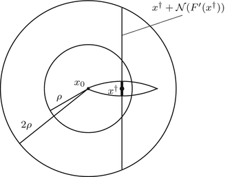
We emphasize that, in general, the limit of the Landweber iterates is no x 0-minimum-norm solution. However, since the monotonicity result of Proposition 2 holds for every solution, the limit of x k has to be at least close to $$x^{\dag }$$. As can be seen below, it has to be the closer the larger ρ can be chosen (Fig. 1).

A183156_2_En_9_Fig1_HTML.gif


Fig. 1
The sketch shows the initial element x 0, the x 0-minimum-norm solution $$x^{\dag }$$, the subset $$x^{\dag } + \mathcal{N}(F^{{\prime}}(x^{\dag }))$$ and in bold the region, where the limit of the iterates x k can be

It is well known that, if y δ does not belong to the range of F, then the iterates $$x_{k}^{\delta }$$ of (13) cannot converge but still allow a stable approximation of a solution of F(x) = y provided the iteration is stopped after k steps. The next result shows that the stopping rule (10), (14) renders the Landweber iteration a regularization method (see [70, Theorem 2.6]):


Theorem 2.

Let the assumptions of Theorem 1 hold and let k = k (δ,y δ ) be chosen according to the stopping rule (10), (14) . Then the Landweber iterates $$x_{k_{{\ast}}}^{\delta }$$ converge to a solution of F(x) = y. If $$\mathcal{N}(F^{{\prime}}(x^{\dag })) \subset \mathcal{N}(F^{{\prime}}(x))$$ for all $$x \in \mathcal{B}_{\rho }(x^{\dag })$$, then $$x_{k_{{\ast}}}^{\delta }$$ converges to $$x^{\dag }$$ as δ → 0.

To obtain convergence rates the exact solution has to satisfy some source conditions. Moreover, one has to guarantee that the iterates remain in $$\mathcal{R}(F^{{\prime}}(x^{\dag })^{{\ast}})$$. In [49] rates were proven under the additional assumption that F satisfies


$$\displaystyle{F^{{\prime}}(x) = R_{ x}F^{{\prime}}(x^{\dag })\quad \mbox{ and}\quad \|R_{ x} - I\| \leq c\|x - x^{\dag }\|,\qquad x \in \mathcal{B}_{ 2\rho }(x_{0})\,,}$$
where $$\{R_{x}\,:\, x \in \mathcal{B}_{2\rho }(x_{0})\}$$ is a family of bounded linear operators $$R_{x}: \mathcal{Y}\rightarrow \mathcal{Y}$$ and c is a positive constant.

Unfortunately, these conditions are not always satisfied (see [49, Example 4.3]). Therefore, we consider instead of (13) the following slightly modified iteration method,


$$\displaystyle{ x_{k+1}^{\delta } = x_{ k}^{\delta } +\omega G^{\delta }(x_{ k}^{\delta })^{{\ast}}(y^{\delta } - F(x_{ k}^{\delta }))\,,\quad k \in \mathbb{N}_{ 0}\,, }$$

(16)
where, as above, $$x_{0}^{\delta } = x_{0}$$ is an initial guess, G δ (x): = G(x, y δ ), and G is a continuous operator mapping $$\mathcal{D}(F) \times \mathcal{Y}$$ into $$\mathcal{L}(\mathcal{X},\mathcal{Y})$$. The iteration will again be stopped according to the discrepancy principle (10).

To obtain local convergence and convergence rates for this modification we need the following assumptions:


Assumption 9.

Let ρ be a positive number such that $$\mathcal{B}_{2\rho }(x_{0}) \subset \mathcal{D}(F)$$.

(i)

The equation F(x) = y has an x 0 -minimum-norm solution $$x^{\dag }$$ in $$\mathcal{B}_{\rho }(x_{0})$$.


(ii)

There exist positive constants c 1, c 2, c 3 and linear operators R x δ such that for all $$x \in \mathcal{B}_{\rho }(x^{\dag })$$ the following estimates hold:


$$\displaystyle{ \|F(x) - F(x^{\dag }) - F^{{\prime}}(x^{\dag })(x - x^{\dag })\| \leq c_{ 1}\|F(x) - F(x^{\dag })\|\|x - x^{\dag }\|\,, }$$

(17)


$$\displaystyle{ G^{\delta }(x) = R_{x}^{\delta }G^{\delta }(x^{\dag })\,, }$$

(18)


$$\displaystyle{ \|R_{x}^{\delta } - I\| \leq c_{ 2}\|x - x^{\dag }\|\,, }$$

(19)


$$\displaystyle{ \|F^{{\prime}}(x^{\dag }) - G^{\delta }(x^{\dag })\| \leq c_{ 3}\delta \,. }$$

(20)


(iii)

The scaling parameter ω in (16) satisfies the condition


$$\displaystyle{\omega \|F^{{\prime}}(x^{\dag })\|^{2} \leq 1\,.}$$


Note that, if instead of (17) the slightly stronger condition


$$\displaystyle\begin{array}{rcl} & & \|F(x) - F(\tilde{x}) - F^{{\prime}}(x)(x -\tilde{ x})\| \leq c\|x -\tilde{ x}\| \\ & & \qquad \|F(x) - F(\tilde{x})\|,x,\tilde{x} \in \mathcal{B}_{2\rho }(x_{0}) \subseteq \mathcal{D}(F),{}\end{array}$$

(21)
holds in $$\mathcal{B}_{2\rho }(x_{0})$$ for some c > 0, then the unique existence of the x 0-minimum-norm solution $$x^{\dag }$$ follows from Proposition 1 if F(x) = y is solvable in $$\mathcal{B}_{\rho }(x_{0})$$.

Convergence and convergence rates for the modification above are obtained as follows (see [70, Theorems 2.8 and 2.13]):


Theorem 3.

Let Assumption 9 hold and let k = k (δ,y δ ) be chosen according to the stopping rule (10).

(i)

If $$\|x_{0} - x^{\dag }\|$$ is so small and if the parameter τ in (10) is so large that


$$\displaystyle{2\eta _{1} +\eta _{ 2}^{2}\eta _{ 3}^{2} < 2}$$

and


$$\displaystyle{\tau > \frac{2(1 +\eta _{1} + c_{3}\eta _{2}\|x_{0} – x^{\dag }\|)} {2 – 2\eta _{1} -\eta _{2}^{2}\eta _{3}^{2}} \,,}$$” src=”/wp-content/uploads/2016/04/A183156_2_En_9_Chapter_Equk.gif”></DIV></DIV></DIV><SPAN class=EmphasisTypeItalic>where</SPAN><br />
<DIV id=Equ23 class=Equation><br />
<DIV class=EquationContent><br />
<DIV class=MediaObject><IMG alt=
then the modified Landweber iterates $$x_{k_{{\ast}}}^{\delta }$$ converge to $$x^{\dag }$$ as δ → 0.


(ii)

If τ > 2 and if $$x^{\dag }- x_{0}$$ satisfies (8) with some 0 < μ ≤ 1∕2 and $$\|v\|$$ sufficiently small, then it holds that


$$\displaystyle{k_{{\ast}} = O\Big(\|v\|^{ \frac{2} {2\mu +1} }\delta ^{- \frac{2} {2\mu +1} }\Big)}$$
and


$$\displaystyle{\|x_{k_{{\ast}}}^{\delta }-x^{\dag }\| = \left \{\begin{array}{ll} o\Big(\|v\|^{ \frac{1} {2\mu +1} }\delta ^{ \frac{2\mu } {2\mu +1} }\Big),&\mu < \frac{1} {2}\,, \\ O\Big(\sqrt{\|v\|\delta }\Big), &\mu = \frac{1} {2}\,.\end{array} \right.}$$


Note that for the modified Landweber iteration we obtain the same convergence rates and the same asymptotical estimate for k as for linear ill-posed problems (compare [36, Theorem 6.5]) if μ ≤ 1∕2 in (8).

Under the Assumption 9 and according to the theorem above the best possible convergence rate is


$$\displaystyle{\|x_{k_{{\ast}}}^{\delta }- x^{\dag }\| = O(\sqrt{\delta })}$$
provided that $$\mu = 1/2$$. Even if μ > 1∕2 we cannot improve this rate without an additional restriction of the nonlinearity of F.

We will show for the following parameter estimation problem that the conditions of Assumption 9 are satisfied if F (x) is replaced by a certain operator G δ (x).


Example 1.

We treat the problem of estimating the diffusion coefficient a in


$$\displaystyle{ \begin{array}{c} - (a(s)u(s)_{s})_{s} = f(s)\,,\quad s \in (0,1)\,,\quad u(0) = 0 = u(1)\,,\end{array} }$$

(22)
where f ∈ L 2; the subscript s denotes derivative with respect to s.

In this example, F is defined as the parameter-to-solution mapping


$$\displaystyle\begin{array}{rcl} F: \mathcal{D}(F):=\{ a \in H^{1}[0,1]\,:\, a(s) \geq \underline{a} > 0\}& \rightarrow & L^{2}[0,1] {}\\ a& \mapsto & F(a):= u(a)\,, {}\\ \end{array}$$” src=”/wp-content/uploads/2016/04/A183156_2_En_9_Chapter_Equ25.gif”></DIV></DIV></DIV>where <SPAN class=EmphasisTypeItalic>u</SPAN>(<SPAN class=EmphasisTypeItalic>a</SPAN>) is the solution of (<SPAN class=InternalRef><A href=22). One can prove that F is Fréchet-differentiable (see, e.g., [24]) with


$$\displaystyle\begin{array}{rcl} F^{{\prime}}(a)h& =& A(a)^{-1}[(hu_{ s}(a))_{s}]\,, {}\\ F^{{\prime}}(a)^{{\ast}}w& =& -B^{-1}[u_{ s}(a)(A(a)^{-1}w)_{ s}]\,, {}\\ \end{array}$$
where


$$\displaystyle\begin{array}{rcl} A(a): H^{2}[0,1] \cap H_{ 0}^{1}[0,1]& \rightarrow & L^{2}[0,1] {}\\ u& \mapsto & A(a)u:= -(au_{s})_{s} {}\\ \end{array}$$
and


$$\displaystyle\begin{array}{rcl} B: \mathcal{D}(B):=\{\psi \in H^{2}[0,1]\,:\,\psi ^{{\prime}}(0) =\psi ^{{\prime}}(1) = 0\}& \rightarrow & L^{2}[0,1] {}\\ \psi & \mapsto & B\psi:= -\psi ^{{\prime\prime}}+\psi \,; {}\\ \end{array}$$
note that B −1 is the adjoint of the embedding operator from H 1[0, 1] in L 2[0, 1].

First of all, we show that F satisfies condition (17): let F(a) = u, $$F(\tilde{a}) =\tilde{ u}$$, and w ∈ L 2. Noting that $$(\tilde{u} - u) \in H^{2} \cap H_{0}^{1}$$ and that A(a) is one-to-one and onto for $$a,\tilde{a} \in \mathcal{D}(F)$$ we obtain that


$$\displaystyle\begin{array}{rcl} & & \langle \,F(\tilde{a}) - F(a) - F^{{\prime}}(a)(\tilde{a} - a),w)\,\rangle _{ L^{2}}\qquad \qquad {}\\ & & \quad =\langle \, (\tilde{u} - u) - A(a)^{-1}[((\tilde{a} - a)u_{ s})_{s}],w\,\rangle _{L^{2}} {}\\ & & \quad =\langle \, A(a)(\tilde{u} - u) - ((\tilde{a} - a)u_{s})_{s},A(a)^{-1}w\,\rangle _{ L^{2}} {}\\ & & \quad =\langle \, ((\tilde{a} - a)(\tilde{u}_{s} - u_{s}))_{s},A(a)^{-1}w\,\rangle _{ L^{2}} {}\\ & & \quad = -\langle \,(\tilde{a} - a)(\tilde{u} - u)_{s},(A(a)^{-1}w)_{ s}\,\rangle _{L^{2}} {}\\ & & \quad =\langle \, F(\tilde{a}) - F(a),((\tilde{a} - a)(A(a)^{-1}w)_{ s})_{s}\,\rangle _{L^{2}}\,. {}\\ \end{array}$$
This together with the fact that $$\|g\|_{L^{\infty }} \leq \sqrt{2}\|g\|_{H^{1}}$$ and that $$\|g\|_{L^{\infty }} \leq \| g^{{\prime}}\|_{L^{2}}$$ if g ∈ H 1 is such that g(ξ) = 0 for some ξ ∈ [0, 1] yields the estimate


$$\displaystyle\begin{array}{rcl} & & \|F(\tilde{a}) - F(a) - F^{{\prime}}(a)(\tilde{a} - a)\|_{ L^{2}}\quad \\ & & \quad \leq \sup _{\|w\|_{ L^{2}}=1}\langle \,F(\tilde{a}) - F(a),((\tilde{a} - a)(A(a)^{-1}w)_{ s})_{s}\,\rangle _{L^{2}} \\ & & \quad \leq \| F(\tilde{a}) - F(a)\|_{L^{2}}\sup _{\|w\|_{ L^{2}}=1}\Big[\Big\|\Big(\frac{\tilde{a} - a} {a} \Big)_{s}\Big\|_{L^{2}}\|a(A(a)^{-1}w)_{ s}\|_{L^{\infty }} \\ & & \qquad +\,\Big\| \frac{\tilde{a} - a} {a} \Big\|_{L^{\infty }}\|w\|_{L^{2}}\Big] \\ & & \quad \leq \underline{a}^{-1}(1 + \sqrt{2} + \underline{a}^{-1}\sqrt{2}\|a\|_{ H^{1}})\|F(\tilde{a}) - F(a)\|_{L^{2}}\|\tilde{a} - a\|_{H^{1}}\,.\qquad {}\end{array}$$

(23)
This implies (17).

The conditions (18) and (19) are not fulfilled with G δ (x) = F (x). Noting that $$F^{{\prime}}(a)^{{\ast}}w$$ is the unique solution of the variational problem: for all v ∈ H 1


$$\displaystyle{ \langle \,(F^{{\prime}}(a)^{{\ast}}w)_{ s},v_{s}\,\rangle _{L^{2}} +\langle \, F^{{\prime}}(a)^{{\ast}}w,v\,\rangle _{ L^{2}} =\langle \, u(a),((A(a)^{-1}w)_{ s}v)_{s}\,\rangle _{L^{2}}\,, }$$

(24)
we propose to choose G δ in (16) as follows: G δ (a) w = G(a, u δ ) w is the unique solution g of the variational problem


$$\displaystyle{ \langle \,g_{s},v_{s}\,\rangle _{L^{2}} +\langle \, g,v\,\rangle _{L^{2}} =\langle \, u^{\delta },((A(a)^{-1}w)_{ s}v)_{s}\,\rangle _{L^{2}}\,,\quad v \in H^{1}\,. }$$

(25)
This operator G δ obviously satisfies (18), since


$$\displaystyle{G(\tilde{a},u^{\delta })^{{\ast}} = G(a,u^{\delta })^{{\ast}}R(\tilde{a},a)^{{\ast}}}$$
with


$$\displaystyle{R(\tilde{a},a)^{{\ast}} = A(a)A(\tilde{a})^{-1}.}$$
The condition (19) is satisfied, since one can estimate as in (23) that


$$\displaystyle{\|R(\tilde{a},a)^{{\ast}}- I\| =\| A(a)A(\tilde{a})^{-1} - I\| \leq \underline{a}^{-1}(1 + \sqrt{2} + \underline{a}^{-1}\sqrt{2}\|\tilde{a}\|_{ H^{1}})\|\tilde{a} - a\|_{H^{1}}\,.}$$
Note that a constant c 2 independent from $$\tilde{a}$$ can be found, since it is assumed that $$\tilde{a} \in \mathcal{B}_{\rho }(a)$$. Now we turn to condition (20): using (24) and (25) we obtain similarly to (23) the estimate


$$\displaystyle\begin{array}{rcl} & & \|(F^{{\prime}}(a)^{{\ast}}- G(a,u^{\delta })^{{\ast}})w\|_{ H^{1}}\, =\,\sup _{\|v\|_{H^{1}}=1}\langle \,u(a) - u^{\delta },((A(a)^{-1}w)_{ s}v)_{s}\,\rangle _{L^{2}}\qquad \qquad {}\\ & & \qquad \leq \underline{a}^{-1}(1 + \sqrt{2} + \underline{a}^{-1}\sqrt{2}\|a\|_{ H^{1}})\|u(a) - u^{\delta }\|_{ L^{2}}\|w\|_{L^{2}}\,. {}\\ \end{array}$$
This together with $$F(a^{\dag }) = u(a^{\dag })$$ and $$\|u^{\delta } - u(a^{\dag })\|_{L^{2}} \leq \delta$$ implies that


$$\displaystyle{\|F^{{\prime}}(a^{\dag }) - G(a^{\dag },u^{\delta })\| \leq \underline{a}^{-1}(1 + \sqrt{2} + \underline{a}^{-1}\sqrt{2}\|a^{\dag }\|_{ H^{1}})\,\delta }$$
and hence (20) holds.

Thus, Theorem 3 is applicable, i.e., if ω and τ are chosen appropriately, then the modified Landweber iterates $$a_{k_{{\ast}}}^{\delta }$$ (cf. (16)) where k is chosen according to the stopping rule (10) converge to the exact solution $$a^{\dag }$$ with the rate $$O(\sqrt{\delta })$$ provided that


$$\displaystyle{a^{\dag }- a_{ 0} = -B^{-1}[u_{ s}(a^{\dag })(A(a^{\dag })^{-1}w)_{ s}]}$$
with $$\|w\|$$ sufficiently small. Note that this means that


$$\displaystyle{\begin{array}{cc} a^{\dag }- a_{o} \in H^{3}\,, &(a^{\dag }- a_{0})_{s}(0) = 0 = (a^{\dag }- a_{0})_{s}(1)\,, \\ z:= \frac{(a^{\dag }- a_{0})_{ss} - (a^{\dag }- a_{0})} {u_{s}(a)} \in H^{1}\,,& \int _{ 0}^{1}z(s)\,ds = 0\,. \end{array} }$$
Basically this means that one has to know all rough parts of $$a^{\dag }$$ up to H 3. But without this knowledge one cannot expect to get the rate $$O(\sqrt{\delta })$$.

In [49] two other nonlinear problems were treated where conditions (18) and (19) are satisfied with G δ (x) = F (x).


Landweber Iteration in Hilbert Scales


We have mentioned in the last subsection that for classical Landweber iteration the rates cannot be better than $$O(\sqrt{\delta })$$ under the given assumptions. However, better rates may be obtained for solutions that satisfy stronger smoothness conditions if the iteration is performed in a subspace of $$\mathcal{X}$$ with a stronger norm. This leads us directly to regularization in Hilbert scales. On the other hand for solutions with poor smoothness properties the number of iterations may be reduced if the iteration is performed in a space with a weaker norm.

First of all, we shortly repeat the definition of a Hilbert scale: let L be a densely defined unbounded self-adjoint strictly positive operator in $$\mathcal{X}$$. Then $$(\mathcal{X}_{s})_{s\in \mathbb{R}}$$ denotes the Hilbert scale induced by L if $$\mathcal{X}_{s}$$ is the completion of $$\bigcap _{k=0}^{\infty }D(L^{k})$$ with respect to the Hilbert space norm $$\|x\|_{s}:=\| L^{s}x\|_{\mathcal{X}}$$; obviously, $$\|x\|_{0} =\| x\|_{\mathcal{X}}$$ (see [78] or [36, Section 8.4] for details).

The operator $$F^{{\prime}}(x_{k}^{\delta })^{{\ast}}$$ in (13) will now be replaced by the adjoint of $$F^{{\prime}}(x_{k}^{\delta })$$ considered as an operator from $$\mathcal{X}_{s}$$ into $$\mathcal{Y}$$. Usually s ≥ 0, but we will see below that there are special cases where a negative choice of s can be advantageous. Since by definition of $$\mathcal{X}_{s}$$ this adjoint is given by $$L^{-2s}F^{{\prime}}(x_{k}^{\delta })^{{\ast}}$$, (13) is replaced by the iteration process


$$\displaystyle{ x_{k+1}^{\delta } = x_{ k}^{\delta } + L^{-2s}F^{{\prime}}(x_{ k}^{\delta })^{{\ast}}(y^{\delta } - F(x_{ k}^{\delta }))\,,\qquad k \in \mathbb{N}_{ 0}\,. }$$

(26)
As in the previous chapter the iteration process is stopped according to the discrepancy principle (10).

Proofs of convergence and convergence rates for this method can be found in [34, 70, 88]. For an approach, where the Hilbert scale is chosen in the space Y, see [33].

The following basic conditions are needed.


Assumption 10.


(i)

$$F: \mathcal{D}(F)(\subset \mathcal{X}) \rightarrow \mathcal{Y}$$ is continuous and Fréchet-differentiable in $$\mathcal{X}$$.


(ii)

F(x) = y has a solution $$x^{\dag }$$.


(iii)

$$\|F^{{\prime}}(x^{\dag })x\| \leq \overline{m}\|x\|_{-a}$$ for all $$x \in \mathcal{X}$$ and some a > 0, $$\overline{m} > 0$$” src=”/wp-content/uploads/2016/04/A183156_2_En_9_Chapter_IEq105.gif”></SPAN>. <SPAN class=EmphasisTypeItalic>Moreover, the extension of</SPAN> <SPAN id=IEq106 class=InlineEquation><IMG alt= to $$\mathcal{X}_{-a}$$ is injective.


(iv)

$$B:= F^{{\prime}}(x^{\dag })L^{-s}$$ is such that $$\|B\|_{\mathcal{X},\mathcal{Y}}\leq 1$$, where − a < s. If s < 0, $$F^{{\prime}}(x^{\dag })$$ has to be replaced by its extension to $$\mathcal{X}_{s}$$.


Usually, for the analysis of regularization methods in Hilbert scales a stronger condition than (iii) is used, namely (cf., e.g., [88])


$$\displaystyle{ \|F^{{\prime}}(x^{\dag })x\| \sim \| x\|_{ -a}\qquad \mbox{ for all}\;\;x \in \mathcal{X}\,, }$$

(27)
where the number a can be interpreted as a degree of ill-posedness of the linearized problem in $$x^{\dag }$$. However, this condition is not always fulfilled. Sometimes one can only prove that condition (iii) in Assumption 10 holds. It might also be possible that one can prove an estimate from below in a slightly weaker norm (see examples in [34]), i.e.,


$$\displaystyle{ \|F^{{\prime}}(x^{\dag })x\| \geq \underline{m}\|x\|_{ -\tilde{a}}\qquad \mbox{ for all }x \in \mathcal{X}\mbox{ and some }\tilde{a} \geq a,\underline{m} > 0\,. }$$” src=”/wp-content/uploads/2016/04/A183156_2_En_9_Chapter_Equ36.gif”></DIV></DIV><br />
<DIV class=EquationNumber>(28)</DIV></DIV></DIV><br />
<DIV class=Para>The next proposition sheds more light onto condition (iii) in Assumption <SPAN class=InternalRef><A href=10 and (28). The proof follows the lines of [36, Corollary 8.22] noting that the results there not only hold for s ≥ 0 but also for s > −a.


Proposition 3.

Let Assumption 10 hold. Then for all ν ∈ [0,1] it holds that


$$\displaystyle\begin{array}{rcl} & \mathcal{D}((B^{{\ast}}B)^{-\frac{\nu }{ 2} }) = \mathcal{R}((B^{{\ast}}B)^{ \frac{\nu }{2} }) \subset \mathcal{X}_{\nu (a+s)}\,, & {}\\ & \|(B^{{\ast}}B)^{ \frac{\nu }{ 2} }x\| \leq \overline{m}^{\nu }\|x\|_{-\nu (a+s)}\qquad \mathrm{for\ all}\quad x \in \mathcal{X}\,, & {}\\ & \|(B^{{\ast}}B)^{-\frac{\nu }{ 2} }x\| \geq \overline{m}^{-\nu }\|x\|_{\nu (a+s)}\qquad \mathrm{for\ all}\quad x \in \mathcal{D}((B^{{\ast}}B)^{-\frac{\nu }{ 2} })\,.\quad & {}\\ \end{array}$$
Note that condition (iii) is equivalent to


$$\displaystyle{\mathcal{R}(F^{{\prime}}(x^{\dag })^{{\ast}}) \subset \mathcal{X}_{ a}\quad {\mathrm{and}}\quad \|F^{{\prime}}(x^{\dag })^{{\ast}}w\|_{ a} \leq \overline{m}\|w\|\quad \mathrm{for\ all}\quad w \in \mathcal{Y}\,.}$$

If in addition condition (28) holds, then for all ν ∈ [0,1] it holds that


$$\displaystyle\begin{array}{rcl} \mathcal{X}_{\nu (\tilde{a}+s)} \subset \mathcal{R}((B^{{\ast}}B)^{ \frac{\nu }{2} }) = \mathcal{D}((B^{{\ast}}B)^{-\frac{\nu }{2} })\,,& & {}\\ \|(B^{{\ast}}B)^{ \frac{\nu }{2} }x\| \geq \underline{m}^{\nu }\|x\|_{-\nu (\tilde{a}+s)}\qquad \mathrm{for\ all}\quad x \in \mathcal{X}\,,& & {}\\ \|(B^{{\ast}}B)^{-\frac{\nu }{2} }x\| \leq \underline{m}^{-\nu }\|x\|_{\nu (\tilde{a}+s)}\qquad \mathrm{for\ all}\quad x \in \mathcal{X}_{\nu (\tilde{a}+s)}\,.& & {}\\ \end{array}$$
Note that condition (28) is equivalent to


$$\displaystyle{\begin{array}{rl} \mathcal{X}_{\tilde{a}} \subset \mathcal{R}(F^{{\prime}}(x^{\dag })^{{\ast}})&{\mathrm{and}}\;\|F^{{\prime}}(x^{\dag })^{{\ast}}w\|_{\tilde{a}} \geq \underline{m}\|w\| \\ &\mathrm{for\ all}\quad w \in \mathcal{N}(F^{{\prime}}(x^{\dag })^{{\ast}})^{\perp }\ {\mathrm{with}}\ F^{{\prime}}(x^{\dag })^{{\ast}}w \in \mathcal{X}_{\tilde{a}}\,.\quad \end{array} }$$

In our convergence analysis the following shifted Hilbert scale will play an important role


$$\displaystyle\begin{array}{rcl} \tilde{\mathcal{X}}_{r}&:=& \mathcal{D}((B^{{\ast}}B)^{ \frac{s-r} {2(a+s)} }L^{s})\quad \mbox{ equipped with the norm} {}\\ \vert \vert \vert x\vert \vert \vert _{r}&:=& \|(B^{{\ast}}B)^{ \frac{s-r} {2(a+s)} }L^{s}x\|_{\mathcal{X}}\,, {}\\ \end{array}$$
where a, s, and B are as in Assumption 10. Some properties of this shifted Hilbert scale can be found in [70, Proposition 3.3].

For the convergence rates analysis we need the following smoothness conditions on the solution $$x^{\dag }$$ and the Fréchet-derivative of F.


Assumption 11.


(i)

$$x_{0} \in \tilde{\mathcal{B}}_{\rho }(x^{\dag }):=\{ x \in \mathcal{X}\,:\, x - x^{\dag }\in \tilde{\mathcal{X}}_{0}\, \wedge \,\vert \vert \vert x - x^{\dag }\vert \vert \vert _{0} \leq \rho \}\subset \mathcal{D}(F)$$ for some ρ > 0.


(ii)

$$\|F^{{\prime}}(x^{\dag }) - F^{{\prime}}(x)\|_{\tilde{\mathcal{X}}_{-b},\mathcal{Y}}\leq c\vert \vert \vert x^{\dag }- x\vert \vert \vert _{0}^{\beta }$$ for all $$x \in \tilde{\mathcal{B}}_{\rho }(x^{\dag })$$ and some b ∈ [0,a], β ∈ (0,1], and c > 0.


(iii)

$$x^{\dag }- x_{0} \in \tilde{\mathcal{X}}_{u}$$ for some $$(a - b)/\beta < u \leq b + 2s$$, i.e., there is an element $$v \in \mathcal{X}$$ so that


$$\displaystyle{L^{s}(x^{\dag }- x_{ 0}) = (B^{{\ast}}B)^{ \frac{u-s} {2(a+s)} }v\quad {\mathrm{and}}\quad \|v\|_{0} = \vert \vert \vert x_{0} - x^{\dag }\vert \vert \vert _{u}\,.}$$


Condition (iii) is a smoothness condition for the exact solution comparable to (8). Usually $$\mathcal{X}_{u}$$ is used instead of $$\tilde{\mathcal{X}}_{u}$$. However, these conditions are equivalent if (27) holds.

For the proof of the next convergence rates result see [70, Theorem 3.8].


Theorem 4.

Let Assumptions 10 and 11 hold. Moreover, let k = k (δ,y δ ) be chosen according to the stopping rule (10) with τ > 2 and let |​|​|x 0 − x |​|​| u be sufficiently small. Then the following estimates are valid for δ > 0 and some positive constants c r:


$$\displaystyle{ k_{{\ast}}\leq \Big ( \frac{2\tau } {\tau -2}\vert \vert \vert x_{0} - x^{\dag }\vert \vert \vert _{ u}\,\delta ^{-1}\Big)^{\frac{2(a+s)} {a+u} } }$$

(29)
and for − a ≤ r < u


$$\displaystyle{\vert \vert \vert x_{k_{{\ast}}}^{\delta }- x^{\dag }\vert \vert \vert _{ r} \leq c_{r}\vert \vert \vert x_{0} - x^{\dag }\vert \vert \vert _{ u}^{\frac{a+r} {a+u} }\delta _{}^{\frac{u-r} {a+u} }\,.}$$

As usual for regularization in Hilbert scales, we are interested in obtaining convergence rates with respect to the norm in $$\mathcal{X} = \mathcal{X}_{0}$$.


Corollary 2.

Under the assumptions of Theorem 4 the following estimates hold:


$$\displaystyle{ \|x_{k_{{\ast}}}^{\delta }- x^{\dag }\| = O\Big(\delta ^{ \frac{u} {a+u} }\Big)\qquad {\mathrm{if}}\quad s \leq 0\,, }$$

(30)


$$\displaystyle{\|x_{k_{{\ast}}}^{\delta }- x^{\dag }\| = O\Big(\|x_{ k_{{\ast}}}^{\delta }- x^{\dag }\|_{ s}\Big) = O\Big(\delta ^{\frac{u-s} {a+u} }\Big)\qquad {\mathrm{if}}\quad 0 < s < u\,.}$$
If in addition (28) holds, then for s > 0 the rate can be improved to


$$\displaystyle{\|x_{k_{{\ast}}}^{\delta }- x^{\dag }\| = O\Big(\vert \vert \vert x_{ k_{{\ast}}}^{\delta }- x^{\dag }\vert \vert \vert _{ r}\Big) = O\Big(\delta ^{\frac{u-r} {a+u} }\Big)\quad {\mathrm{if}}\quad r:= \frac{s(\tilde{a}-a)} {\tilde{a}+s} \leq u\,.\quad }$$

Note that (29) implies that k is finite for δ > 0 and hence $$x_{k_{{\ast}}}^{\delta }$$ is a stable approximation of $$x^{\dag }$$.

Moreover, it can be seen from (29) that the larger s the faster k possibly grows if δ → 0. As a consequence, s should be kept as small as possible to reduce the number of iterations and hence to reduce the numerical effort. If u is close to 0, it might be possible to choose a negative s. According to (30), we would still get the optimal rate, but, due to (29), k would not grow so fast. Choosing a negative s could be interpreted as a preconditioned Landweber method (cf. [34]).

We will now comment on the rates in Corollary 2: if only Assumption 10 (iii) is satisfied, i.e., if $$\|F^{{\prime}}(x^{\dag })x\|$$ may be estimated through the norm in $$\mathcal{X}_{-a}$$ only from above, convergence rates in $$\mathcal{X}$$ can only be given if s < u, i.e., only for the case of undersmoothing. If s > 0, the rates will not be optimal in general. To obtain rates also for s > u, i.e., for the case of oversmoothing, condition (28

Only gold members can continue reading. Log In or Register to continue

Stay updated, free articles. Join our Telegram channel

Apr 9, 2016 | Posted by in GENERAL RADIOLOGY | Comments Off on Solution Methods

Full access? Get Clinical Tree

Get Clinical Tree app for offline access